radiatR

if (requireNamespace("pkgload", quietly = TRUE)) {
  # Always load from source so the vignette reflects the current development state.
  pkgload::load_all("../..", export_all = FALSE, helpers = FALSE, quiet = TRUE)
} else if (requireNamespace("radiatR", quietly = TRUE)) {
  library(radiatR)
} else {
  stop("Package 'radiatR' not installed and 'pkgload' not available.")
}
library(ggplot2)

Overview

radiatR streamlines the journey from headings and trajectories on the unit disk to publication-ready radial plots. Angles can be supplied directly, or reconstructed from movement trajectories. The package includes:

• utilities for importing paired landmark/track text files produced by popular tracking suites;
• helpers for extracting trial limits and computing circular summary statistics;
• polished ggplot2 layers for drawing concentric guides and annotated paths.

Prefer a point-and-click interface? launch_app() opens an interactive Shiny companion to upload tracks or headings, configure the analysis, and view the figures together with the radiatR code that reproduces them.

launch_app()

Import Pipeline

The package ships a full set of example tracks (a millipede orientation experiment) that demonstrate the import workflow. Landmark files (_point01.txt) record two pixel-space reference points per trial (the origin and a target location on the circumference); track files (_point02.txt) contain the full xy trajectory. The files ship as one archive, unpacked here into a temporary directory.

untar(system.file("extdata", "tracks.tar.gz", package = "radiatR"),
      exdir = tempdir())
track_dir     <- file.path(tempdir(), "tracks")
manifest_path <- system.file("extdata", "millipede_trials.csv", package = "radiatR")

file_tbl  <- import_tracks(track_dir)
manifest  <- import_info(manifest_path)

ts_demo <- suppressWarnings(get_all_object_pos(file_tbl = file_tbl, track_dir = track_dir,
                                               manifest = manifest))
#> 478 points across 106 trials exceeded the unit circle boundary (radius > 1); coordinates left unscaled.
ts_demo
#> Tracks: 235 trajectories, 44331 observations
#> Columns: id='trial_id', time='frame', angle='rel_theta' (radians), x='trans_x', y='trans_y', rel_x='rel_x', rel_y='rel_y'
#> Transform steps: unit_circle_mapping 
#> # A tibble: 6 × 10
#>   trial_id frame     x     y trans_x  trans_y rel_theta video order vid_ord
#>   <chr>    <dbl> <dbl> <dbl>   <dbl>    <dbl>     <dbl> <chr> <chr> <chr>  
#> 1 10_1_1       1  456.  372. 0.00511  0           6.21  10_1  1     10_1_1 
#> 2 10_1_1       2  458.  370. 0.0128   0.00770     0.464 10_1  1     10_1_1 
#> 3 10_1_1       3  456.  370. 0.00511  0.00770     0.908 10_1  1     10_1_1 
#> 4 10_1_1       4  454.  370. 0        0.00770     1.49  10_1  1     10_1_1 
#> 5 10_1_1       5  456.  377. 0.00511 -0.0153      4.96  10_1  1     10_1_1 
#> 6 10_1_1       6  459.  382. 0.0154  -0.0307      5.10  10_1  1     10_1_1

get_all_object_pos() reads each landmark/track pair, normalises coordinates to a unit circle (radius = 1), and returns a Tracks. Trial metadata (physical radius, target position, frame limits) is in ts_demo@meta$trial_limits.

Full Millipede Dataset

The package also provides cpunctatus, a pre-computed Tracks of all 235 Cylindroiulus punctatus trajectories across the stimulus conditions (target half-widths of 5, 10, 15, 20, 30, 40, 50 degrees, plus a featureless control with arc = 0). Loading it is instant, and the per-trial target half-width is already attached as the arc column.

data(cpunctatus)
cpunctatus
#> Tracks: 235 trajectories, 44331 observations
#> Columns: id='trial_id', time='frame', angle='rel_theta' (radians), x='trans_x', y='trans_y', rel_x='rel_x', rel_y='rel_y'
#> Transform steps: unit_circle_mapping 
#> # A tibble: 6 × 18
#>   trial_id frame     x     y trans_x  trans_y trans_rho abs_theta rel_theta
#>   <chr>    <int> <dbl> <dbl>   <dbl>    <dbl>     <dbl>     <dbl>     <dbl>
#> 1 10_1_1       1  456.  372. 0.00511  0         0.00511     0         6.21 
#> 2 10_1_1       2  458.  370. 0.0128   0.00770   0.0149      0.541     0.464
#> 3 10_1_1       3  456.  370. 0.00511  0.00770   0.00924     0.985     0.908
#> 4 10_1_1       4  454.  370. 0        0.00770   0.00770     1.57      1.49 
#> 5 10_1_1       5  456.  377. 0.00511 -0.0153    0.0162      5.03      4.96 
#> 6 10_1_1       6  459.  382. 0.0154  -0.0307    0.0343      5.18      5.10 
#> # ℹ 9 more variables: rel_x <dbl>, rel_y <dbl>, video <chr>, order <chr>,
#> #   vid_ord <chr>, radius <dbl>, arc <ord>, type <chr>, individual <chr>

Plotting Trajectories

radiate() draws trajectories on a unit circle with concentric reference rings. Colouring by the arc factor shows how paths cluster by condition.

radiate(cpunctatus,
        group_col  = "trial_id",
        colour_col = "arc",
        show_labels = FALSE,
        show_arrow  = FALSE,
        display    = circ_display(zero = 0))
#> Warning: Removed 105 rows containing missing values or values outside the scale range
#> (`geom_path()`).

By default radiate() plots the landmark-relative frame — each trajectory rotated so its trial landmark (e.g. the stimulus) sits at the same direction. To inspect the un-rotated frame as an experimental control (for instance, to check the apparatus carries no directional bias of its own), pass coords = "absolute":

radiate(cpunctatus, coords = "absolute")
#> Warning: Removed 105 rows containing missing values or values outside the scale range
#> (`geom_path()`).

The circumference can be labelled in domain units instead of degrees — useful for time-of-year or compass data. angle_labels selects a built-in scale and aligns the tick count to it:

radiate(cpunctatus, angle_labels = "months")
#> Warning: Removed 105 rows containing missing values or values outside the scale range
#> (`geom_path()`).

The other built-in scales are "cardinal" (compass), "hours" (24-hour clock), and "seconds". For finer control — an 8-point compass, a 12-hour clock, different month formats — add an explicit circumference_labs() layer built from scale_cardinal(), scale_clock(), scale_months(), or scale_seconds():

radiate(cpunctatus, ticks = FALSE, show_labels = FALSE, show_arrow = FALSE) +
  circumference_labs(scale_clock(hours = 12))
#> Warning: Removed 105 rows containing missing values or values outside the scale range
#> (`geom_path()`).

n_labels sets how many equally-spaced ticks and numeric labels to draw — e.g. 12 for a clock face, 4 for cardinals only, 0 for a bare circle — and angle_label_position places the numeric labels "outside" (default), "inside", or "split" (cardinals inside, diagonals outside):

radiate(cpunctatus, n_labels = 12, angle_label_position = "split",
        show_labels = FALSE, show_arrow = FALSE)
#> Warning: Removed 105 rows containing missing values or values outside the scale range
#> (`geom_path()`).

Reference frame: relative vs absolute

By default radiate() plots the landmark-relative frame: each trajectory is rotated so its trial landmark (e.g. the stimulus) sits at the same direction. Pass coords = "absolute" to plot the absolute (native) frame instead — useful as an experimental control, for instance to check the apparatus carries no directional bias of its own. (set_reference() sets the per-trajectory landmark direction that defines the relative frame.)

radiate(cpunctatus, coords = "absolute")
#> Warning: Removed 105 rows containing missing values or values outside the scale range
#> (`geom_path()`).

Colour tracks by position

Setting track_colour = "sequence" shades each path along its own length, so the direction of travel reads at a glance: a per-track gradient from start (dark) to finish (bright), with a continuous “start → finish” colourbar. This mode owns the colour aesthetic, so it is not combined with colour_col/colour_cycle.

# colour each track from start (dark) to finish (bright)
radiate(cpunctatus, show_tracks = TRUE, track_colour = "sequence")
#> Warning: Removed 105 rows containing missing values or values outside the scale range
#> (`geom_path()`).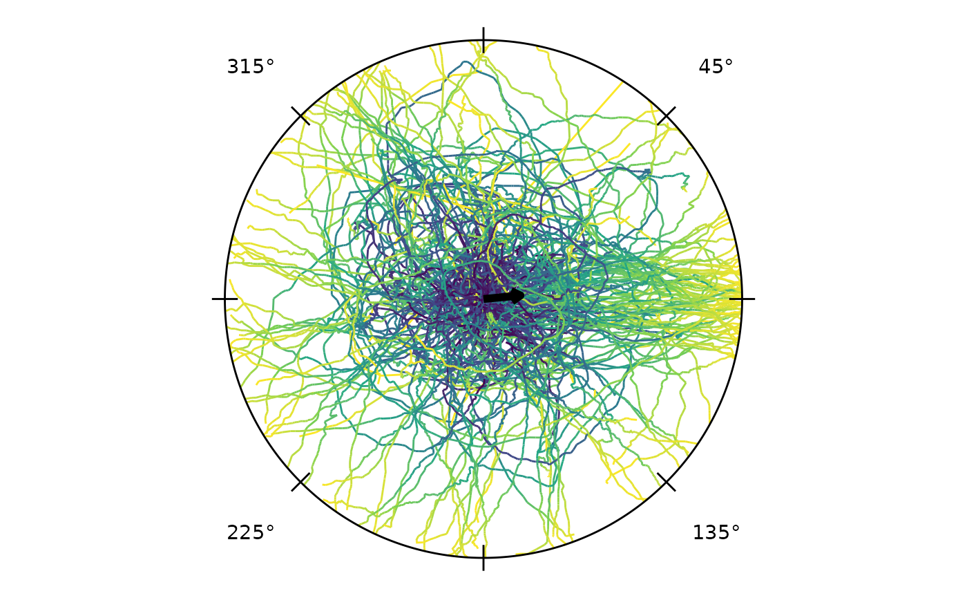

Representing time

Attach a capture frame rate (frames per second) to a Tracks object and the time aspect of frame-indexed tracks can be reported in real seconds and shown on the plot. The frame rate is stored in the object’s metadata; the time/frame column itself is never altered. track_duration() reports the elapsed seconds of each trajectory, and track_colour = "time" colours each path by elapsed time (POSIXct time works without a frame rate).

# attach a capture rate, then represent the time aspect
ts <- set_frame_rate(cpunctatus, fps = 30)
head(track_duration(ts))                                 # seconds per track
#>        id  duration
#> 1  10_1_1 2.6666667
#> 2 10_10_1 9.9333333
#> 3 10_11_1 2.1333333
#> 4 10_12_1 1.5666667
#> 5 10_13_1 2.6333333
#> 6 10_14_1 0.9666667
radiate(ts, show_tracks = TRUE, track_colour = "time")   # colour by elapsed time
#> Warning: Removed 105 rows containing missing values or values outside the scale range
#> (`geom_path()`).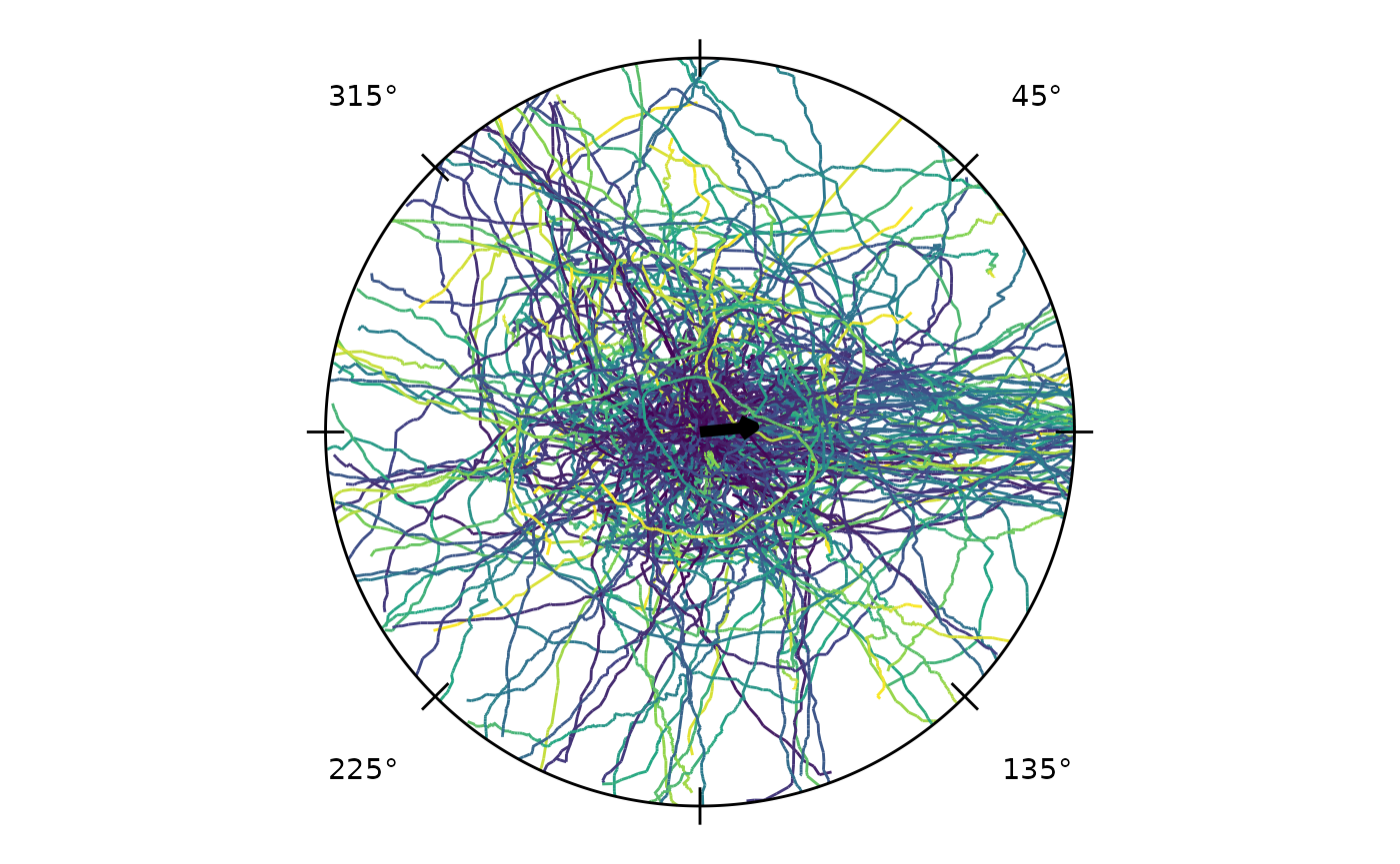

A frame rate also lets track_speed() report each trajectory’s speed in real units. With the default unit-circle coordinates that is radii per second.

# speed in radii per second once a frame rate is set
ts <- set_frame_rate(cpunctatus, fps = 30)
head(track_speed(ts))            # mean speed per track
#>         trial_id     speed
#> 10_1_1    10_1_1 0.5117093
#> 10_10_1  10_10_1 0.8797423
#> 10_11_1  10_11_1 0.5992307
#> 10_12_1  10_12_1 0.7900211
#> 10_13_1  10_13_1 0.6047888
#> 10_14_1  10_14_1 0.9688229
head(track_speed(ts, stat = "max"))
#>         trial_id     speed
#> 10_1_1    10_1_1 0.9965993
#> 10_10_1  10_10_1 2.6559596
#> 10_11_1  10_11_1 1.3979594
#> 10_12_1  10_12_1 1.2717587
#> 10_13_1  10_13_1 1.3794944
#> 10_14_1  10_14_1 1.4268880

The same frame rate lets radiate() colour each path by its instantaneous speed, the per-observation sibling of track_speed().

# colour each path by its instantaneous speed (needs a frame rate)
ts <- set_frame_rate(cpunctatus, fps = 30)
radiate(ts, show_tracks = TRUE, track_colour = "speed")
#> Warning: Removed 105 rows containing missing values or values outside the scale range
#> (`geom_path()`).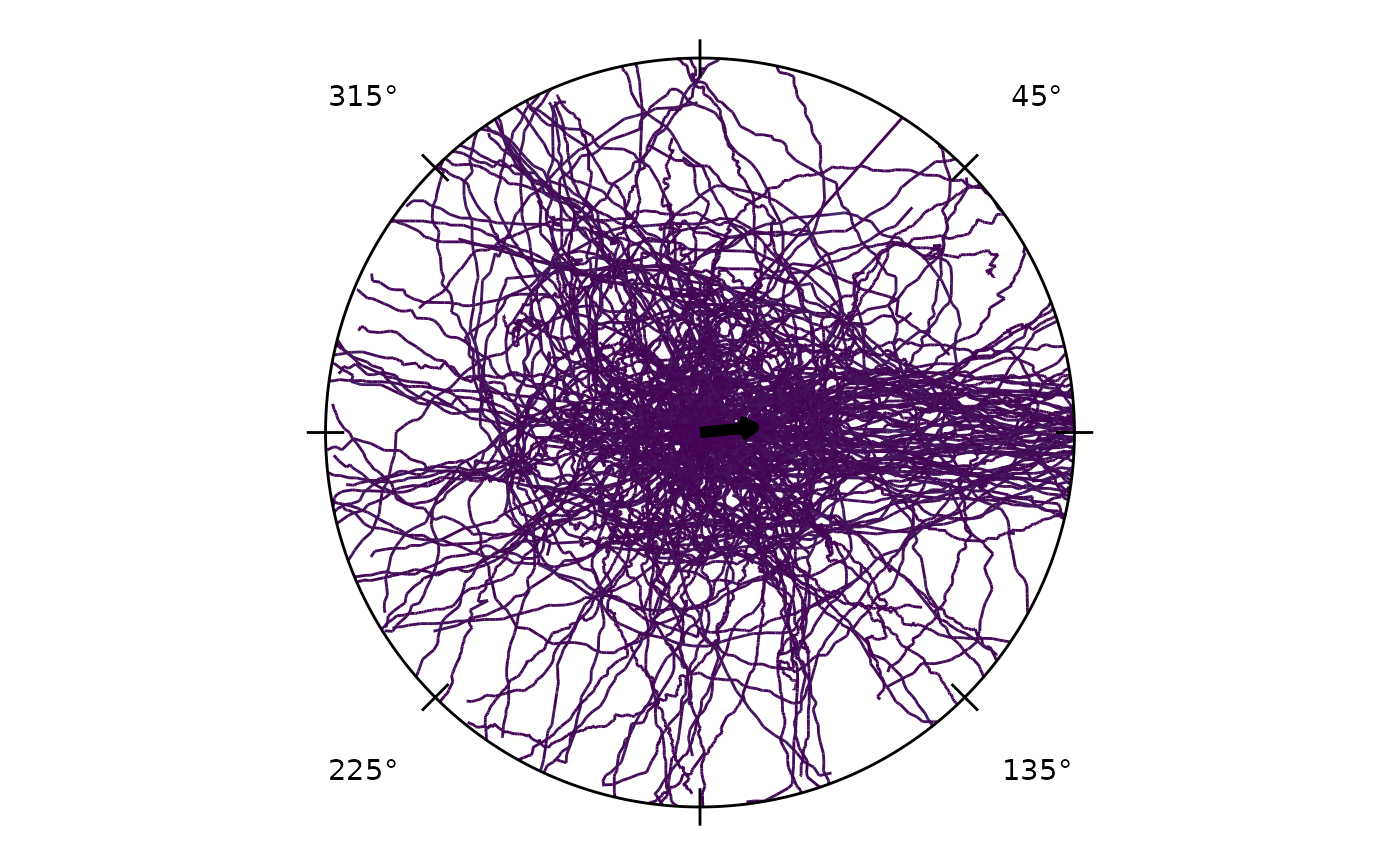

If you know a physical scale, calibrate distances so lengths and speeds report in real units. The scale is physical units per coordinate unit (e.g. mm per radius); unset, everything stays in coordinate units (radii).

# calibrate distance (optional): 50 mm per coordinate unit (radius)
ts <- set_distance_scale(set_frame_rate(cpunctatus, 30), 50, unit = "mm")
head(track_length(ts))      # path length per track, in mm
#>         trial_id    length
#> 10_1_1    10_1_1  68.22790
#> 10_10_1  10_10_1 436.93869
#> 10_11_1  10_11_1  63.91794
#> 10_12_1  10_12_1  61.88499
#> 10_13_1  10_13_1  79.63053
#> 10_14_1  10_14_1  46.82644
head(track_speed(ts))       # mean speed per track, in mm/s
#>         trial_id    speed
#> 10_1_1    10_1_1 25.58546
#> 10_10_1  10_10_1 43.98712
#> 10_11_1  10_11_1 29.96154
#> 10_12_1  10_12_1 39.50105
#> 10_13_1  10_13_1 30.23944
#> 10_14_1  10_14_1 48.44115
# or from two measured landmarks:
# ts <- calibrate_distance(ts, coord_distance = 0.8, real_distance = 40, unit = "mm")

A frame rate also unlocks per-observation kinematics: velocity_vector() gives the velocity components (vx, vy; distance-calibrated when a scale is set) and angular_velocity() the signed turning rate (counter-clockwise positive).

# velocity components and turning rate (need a frame rate; vx/vy use the distance scale)
ts <- set_frame_rate(cpunctatus, fps = 30)
head(velocity_vector(ts))                 # vx, vy per observation
#>           vx         vy
#> 1         NA         NA
#> 2  0.2309549  0.2309549
#> 3 -0.2309549  0.0000000
#> 4 -0.1533230  0.0000000
#> 5  0.1533230 -0.6909238
#> 6  0.3076164 -0.4599689
head(angular_velocity(ts, units = "degrees"))   # turning rate, deg/s (CCW +)
#> [1]        NA 4050.0000    0.0000 3075.3530  637.8571    0.0000

velocity_angle() gives the direction of travel at each observation, in the same convention as headings — so it feeds straight into the circular tools:

ts <- set_frame_rate(cpunctatus, fps = 30)
head(velocity_angle(ts, units = "degrees"))   # movement direction per observation
#> [1]       NA  45.0000 180.0000 180.0000 282.5118 303.7737

Reduced to one row per track, track_velocity() gives each path’s net (average) velocity vector and track_turning() summarises its turning rate.

# per-track summaries (need a frame rate; velocity uses the distance scale)
ts <- set_frame_rate(cpunctatus, fps = 30)
head(track_velocity(ts))                       # net velocity vector (vx, vy) per track
#>         trial_id           vx          vy
#> 10_1_1    10_1_1  0.244467664  0.27514439
#> 10_10_1  10_10_1  0.001745265 -0.08705181
#> 10_11_1  10_11_1  0.072856469  0.47347488
#> 10_12_1  10_12_1 -0.411668880  0.50517999
#> 10_13_1  10_13_1  0.000000000 -0.38637420
#> 10_14_1  10_14_1 -0.461499359  0.78038925
head(track_turning(ts, units = "degrees"))     # typical turning rate (deg/s) per track
#>         trial_id   turning
#> 10_1_1    10_1_1 1122.7526
#> 10_10_1  10_10_1  603.2629
#> 10_11_1  10_11_1 1019.2704
#> 10_12_1  10_12_1  878.3579
#> 10_13_1  10_13_1  913.2823
#> 10_14_1  10_14_1  351.5319

For a non-circular view, plot_profile() draws a per-observation kinematics metric — instantaneous speed or turning rate — against elapsed time, one line per track. It is the ggplot sibling of radiate().

# speed (or turning rate) along each track over time
ts <- set_frame_rate(cpunctatus, fps = 30)
plot_profile(ts, metric = "speed")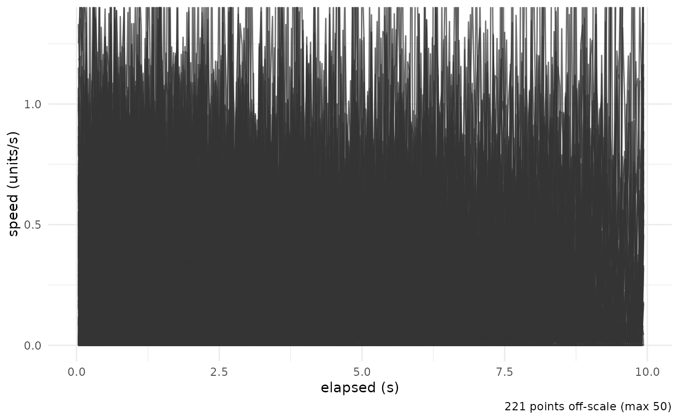

plot_profile(ts, metric = "turning", units = "degrees")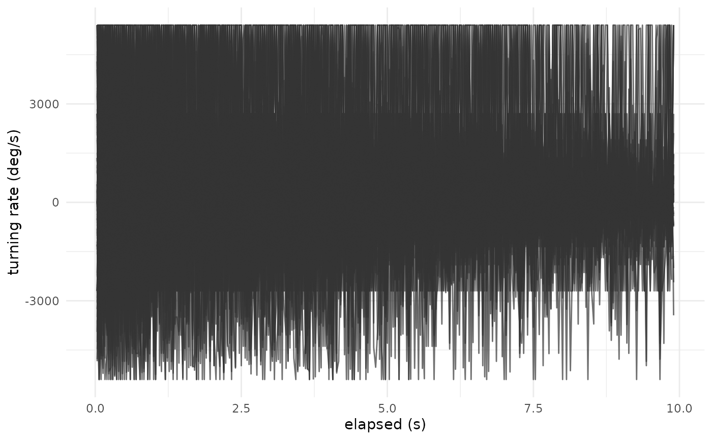

metric = "direction" plots the movement direction over time (as points, since direction is circular):

plot_profile(ts, metric = "direction", units = "degrees")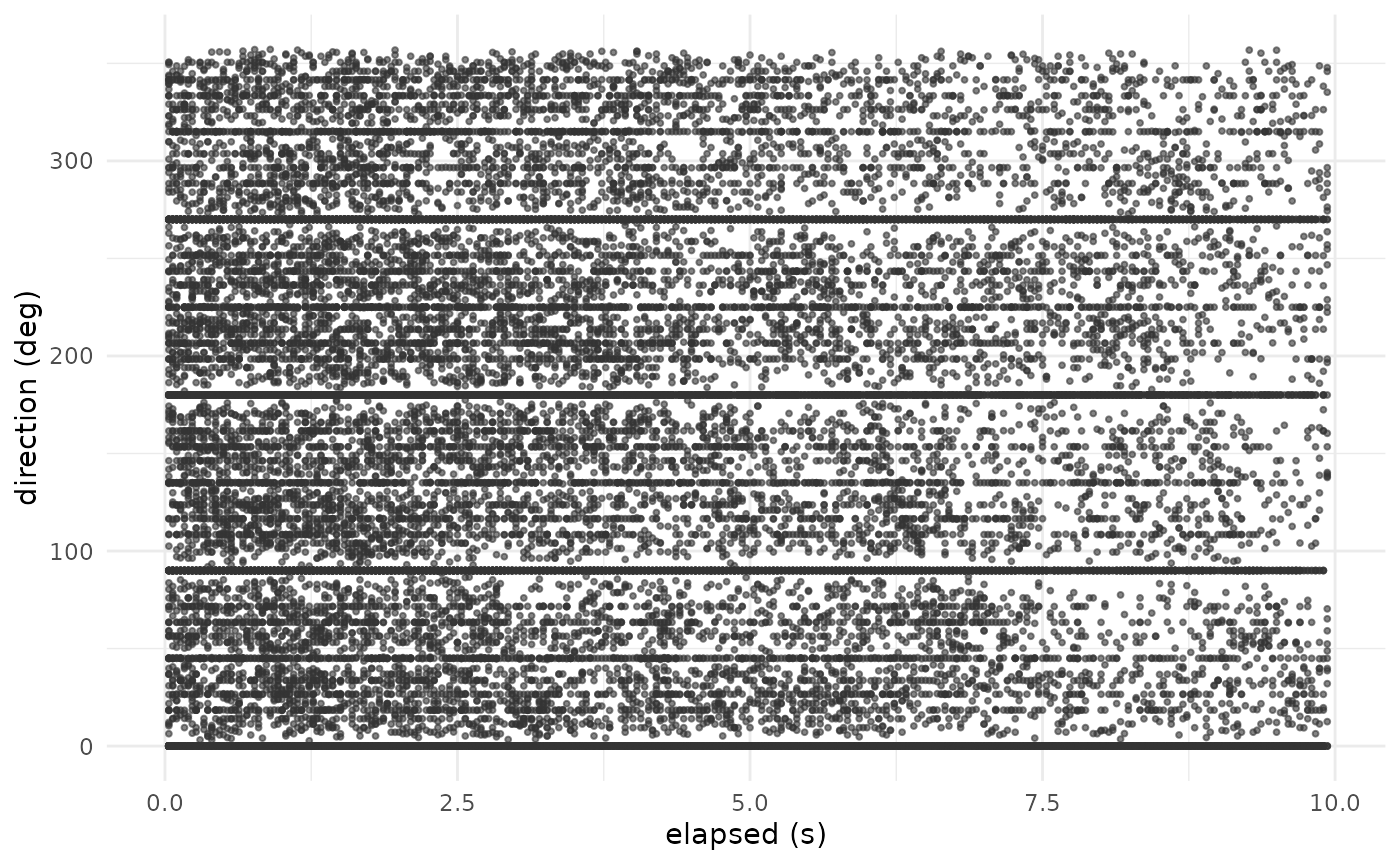

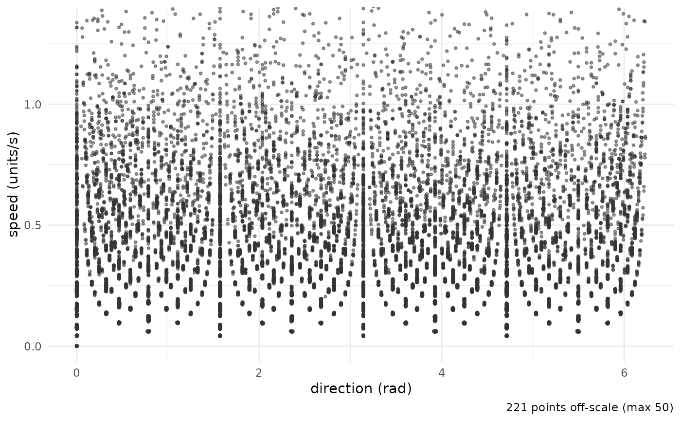
plot_speed_direction() crosses the two — each observation’s speed against its movement direction. The speed axis is robustly clipped by default so a few single-frame tracking artifacts do not crush the display:

plot_speed_direction(ts)

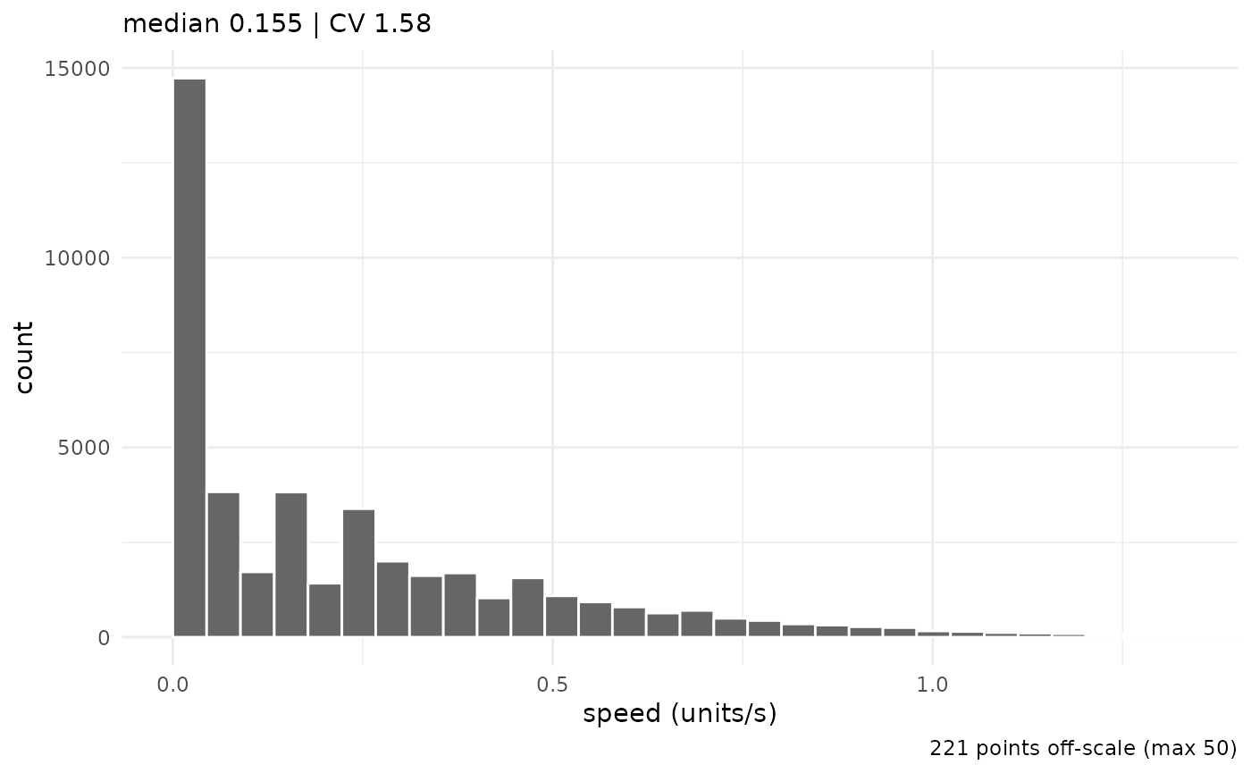
The pooled speed distribution, with median and CV, comes from plot_speed_histogram():

plot_speed_histogram(ts)

Heading Overlays

The crossing method — projecting the vector between two concentric-ring crossings to the unit circle — assigns one directional heading per trial. derive_headings() with return_coords = TRUE returns both the heading angle and the inner-ring crossing position.

hd <- derive_headings(cpunctatus, rule = "crossing",
                      circ0 = 0.2, circ1 = 0.4,
                      return_coords = TRUE)
#> Warning: derive_headings(rule = 'crossing'): 25 of 251 headings (10.0%), from
#> 25 of 235 trials, are missing and are excluded from circular statistics.
#> Rule-based failures are often non-random and can bias results; inspect attr(x,
#> "missing_ids").
names(hd)[names(hd) == "id"] <- "trial_id"
# join the target half-width (arc) from the dataset for grouping/faceting
arc_map <- unique(cpunctatus@data[, c("trial_id", "arc")])
hd       <- merge(hd, arc_map, by = "trial_id")
hd$arc   <- factor(hd$arc)
attr(hd, "colour_col") <- "arc"
attr(hd, "display")    <- circ_display(zero = 0)
head(hd[, c("trial_id", "arc", "heading", "x_inner", "y_inner")])
#>   trial_id arc   heading     x_inner     y_inner
#> 1   10_1_1  10 0.3545811  0.19556350 -0.04102813
#> 2  10_10_1  10 6.2337825 -0.03715972  0.19558015
#> 3  10_11_1  10 1.3353505 -0.07231344  0.18624466
#> 4  10_12_1  10 2.2846471 -0.18291981  0.08084798
#> 5  10_13_1  10 5.6521348  0.18223038  0.08232129
#> 6  10_14_1  10 1.6589765  0.09025066  0.17836615

Overlaying the heading endpoints (one hollow circle per trial) and the grand mean direction on the combined trajectory plot gives a compact summary of the full dataset:

p_all <- radiate(cpunctatus,
                 group_col   = "trial_id",
                 colour_col  = "arc",
                 show_labels = FALSE,
                 show_arrow  = FALSE,
                 display     = circ_display(zero = 0)) +
  add_heading_points(hd, colour_col = "arc", size = 1, alpha = 0.6)

p_all + add_heading_arrow(hd)
#> Warning: Removed 105 rows containing missing values or values outside the scale range
#> (`geom_path()`).
#> Warning: Removed 25 rows containing missing values or values outside the scale range
#> (`geom_point()`).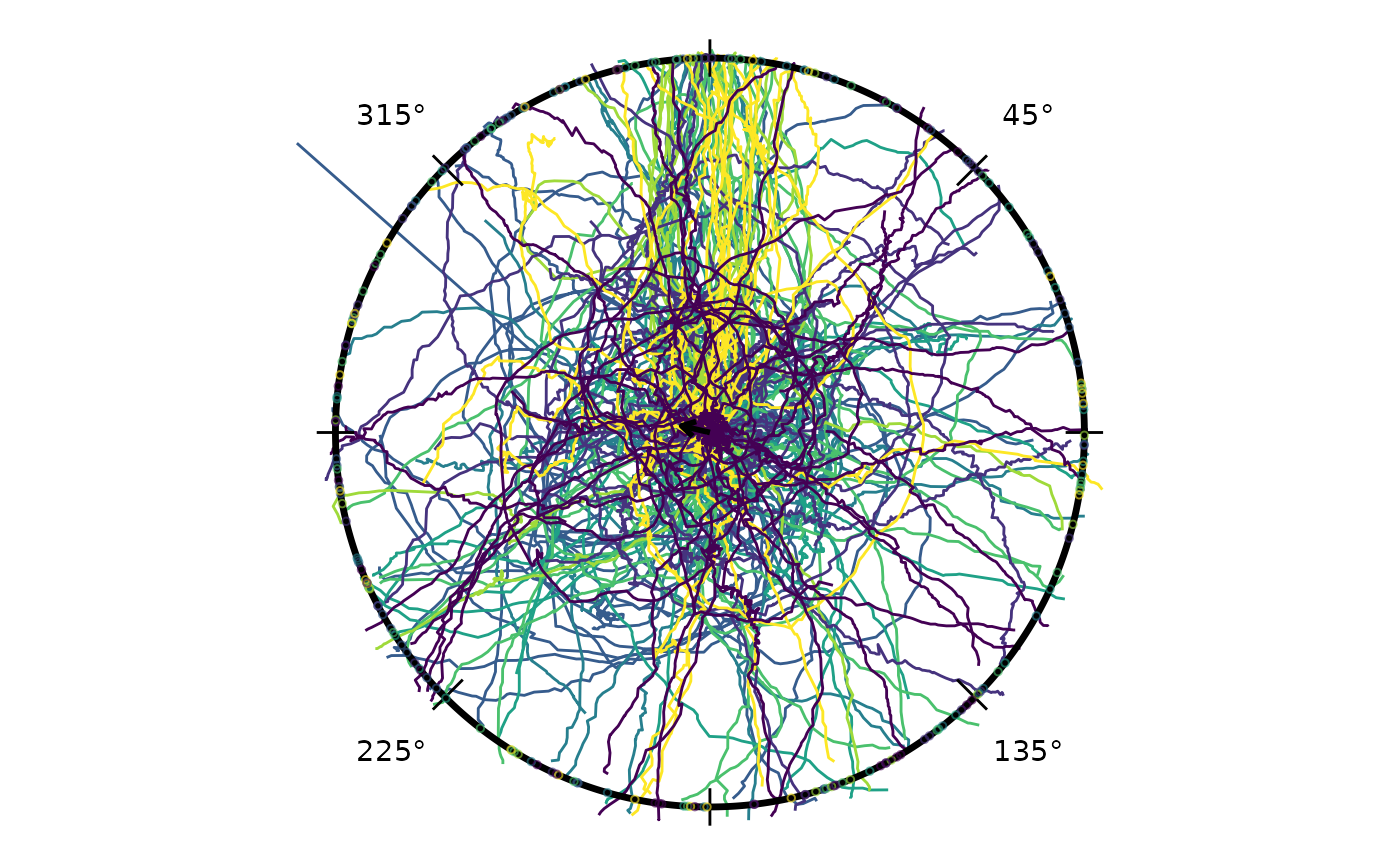

The grand mean arrow points at 283.2° relative to the reference direction (clock convention; 0° = toward reference) with R = 0.08, reflecting the overall reference-relative tendency across all conditions.

Circular Interval Arc

Three functions handle directional uncertainty arcs in parallel with the density overlay functions:

Function	Role
compute_circ_interval()	Computes arc bounds from raw headings; returns a data frame with lower, upper, mean_dir, and wraps
add_circ_interval()	Renders any bounds data frame as an arc at a configurable radius — agnostic to how the bounds were produced
add_heading_interval()	Convenience wrapper: calls the two above in sequence

Two statistics are supported: stat = "bootstrap_ci" bootstraps the von Mises MLE confidence interval for the mean direction; stat = "sd" draws a ±1 circular SD arc. The split design lets you substitute Bayesian credible bounds into the data frame before rendering:

iv <- compute_circ_interval(hd, group_col = "arc", stat = "bootstrap_ci")
# replace with Bayesian posteriors: iv$lower <- ...; iv$upper <- ...
add_circ_interval(iv, colour_col = "arc")

Building Up a Panel

Layers compose with the standard ggplot2 + operator, so a plot can be assembled feature by feature. The four chunks below start from trajectories only and add heading endpoints, the grand mean arrow, and finally a bootstrap CI arc.

Trajectories:

p <- radiate(cpunctatus,
             group_col   = "trial_id",
             colour_col  = "arc",
             show_labels = FALSE,
             show_arrow  = FALSE,
             display     = circ_display(zero = 0))
p
#> Warning: Removed 105 rows containing missing values or values outside the scale range
#> (`geom_path()`).

+ Heading endpoints at each trial’s crossing location:

p <- p + add_heading_points(hd, colour_col = "arc", size = 1.5, alpha = 0.7)
p
#> Warning: Removed 105 rows containing missing values or values outside the scale range
#> (`geom_path()`).
#> Warning: Removed 25 rows containing missing values or values outside the scale range
#> (`geom_point()`).

+ Grand mean direction arrow:

p <- p + add_heading_arrow(hd)
p
#> Warning: Removed 105 rows containing missing values or values outside the scale range
#> (`geom_path()`).
#> Warning: Removed 25 rows containing missing values or values outside the scale range
#> (`geom_point()`).

The arc at radius 1.05 spans the 95 % bootstrap confidence interval for the grand mean direction pooled across all arc conditions.

Circular Boxplot

add_circular_boxplot() overlays a Tukey-like boxplot for circular data (Buttarazzi, Pandolfo & Porzio, 2018): the box spans the central 50 % around the circular median, whiskers reach a concentration-adjusted fence, and far-out values are marked individually. It composes onto a radiate() plot like the other overlay helpers.

radiate(cpunctatus) + add_circular_boxplot(hd)
#> Warning: Removed 105 rows containing missing values or values outside the scale range
#> (`geom_path()`).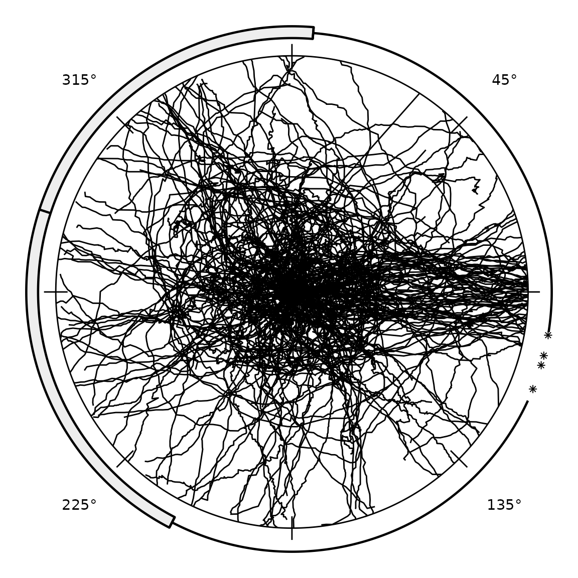

circ_boxplot_stats() returns the underlying numeric summary — the circular median, box hinges, fences, far-out values, and the closed-form von Mises fence multiplier — so the boxplot can be inspected or reproduced independently of the plot:

circ_boxplot_stats(hd)$constant
#> [1] 0.5995206

The boxplot is not recommended for uniform or multimodal data: with no clear central direction the box spans roughly half the circle and the summary is uninformative. circ_boxplot_stats() flags such cases via its drawable and reason fields, and add_circular_boxplot() emits a warning rather than drawing a misleading box. Position-based axial data is supported via axial = TRUE, which draws the box and whiskers at both poles of the median axis.

Colour Options

Three strategies control how trajectories are coloured.

Option 1 — single colour. Pass a colour string directly to the heading-overlay helpers; omit colour_col from radiate() to draw all tracks in the default grey.

Option 2 — cycling palette. colour_cycle assigns each trajectory a colour index that cycles back to 1 after every n trajectories. When facets is set the cycle restarts independently within each panel so that trajectory 1 in every panel always gets colour 1. Pass an integer for automatic palette assignment, or a character vector to specify colours explicitly.

Option 3 — variable mapping. colour_col maps any data column to colour (e.g. the arc factor used in the combined-trajectory plot above).

Per-Condition Panels

Faceting by arc angle shows each condition separately. Within each panel, assign_cycle_colours() distinguishes individual trajectories by cycling through 10 colours, resetting at each panel boundary. Calling it explicitly on both the track data and the headings data frame (joining by trial id) means heading markers inherit the exact per-trajectory colour — not a single per-condition colour — when colour_col is used for both.

# Pre-compute cycling colours: 10 colours, restarting within each arc panel.
# Join to headings so heading layers can use the same column.
cpunctatus_cc        <- cpunctatus
cpunctatus_cc@data   <- assign_cycle_colours(cpunctatus@data,
                                            id_col    = "trial_id",
                                            n         = 10,
                                            panel_col = "arc")
colour_map <- unique(cpunctatus_cc@data[, c("trial_id", "cycle_colour")])
hd_cc      <- merge(hd, colour_map,
                    by      = "trial_id", all.x = TRUE)
attr(hd_cc, "display")    <- attr(hd, "display", exact = TRUE)
attr(hd_cc, "colour_col") <- "cycle_colour"

p <- radiate(cpunctatus_cc,
        group_col    = "trial_id",
        colour_col   = "cycle_colour",
        facets     = "arc",
        ncol         = 3,
        show_labels  = FALSE,
        show_arrow   = FALSE,
        display      = circ_display(zero = 0))
p
#> Warning: Removed 105 rows containing missing values or values outside the scale range
#> (`geom_path()`).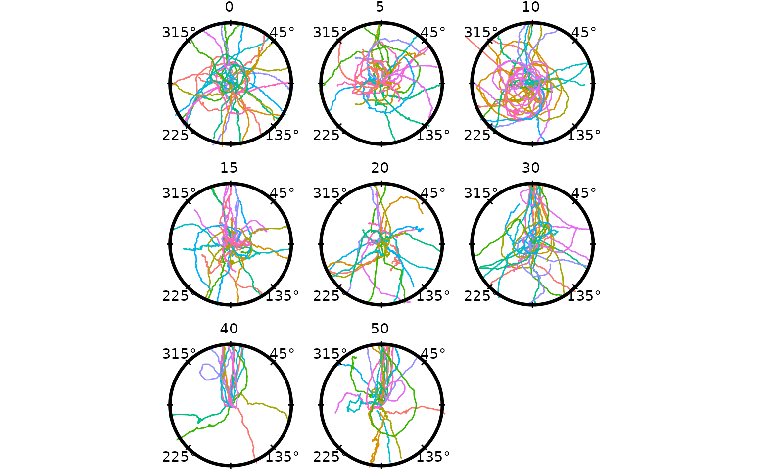

For a two-way layout, rows and cols facet into a grid via ggplot2::facet_grid() (mirroring ggplot — each takes one or more columns):

radiate(cpunctatus, group_col = "trial_id", rows = "type", cols = "arc")

Use rows/cols (grid) or facets (wrap), not both.

+ Bootstrap CI arc added first so it sits behind heading markers:

p <- p + add_heading_interval(hd_cc, group_col = "arc", colour = "black",
                               stat = "bootstrap_ci", boot_reps = 999L)
p
#> Warning: Removed 105 rows containing missing values or values outside the scale range
#> (`geom_path()`).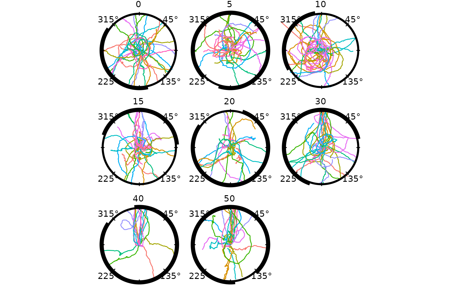

+ Heading vectors (dotted lines from inner crossing to the circumference):

p <- p + add_heading_vectors(hd_cc)
p
#> Warning: Removed 105 rows containing missing values or values outside the scale range
#> (`geom_path()`).
#> Warning: Removed 25 rows containing missing values or values outside the scale range
#> (`geom_segment()`).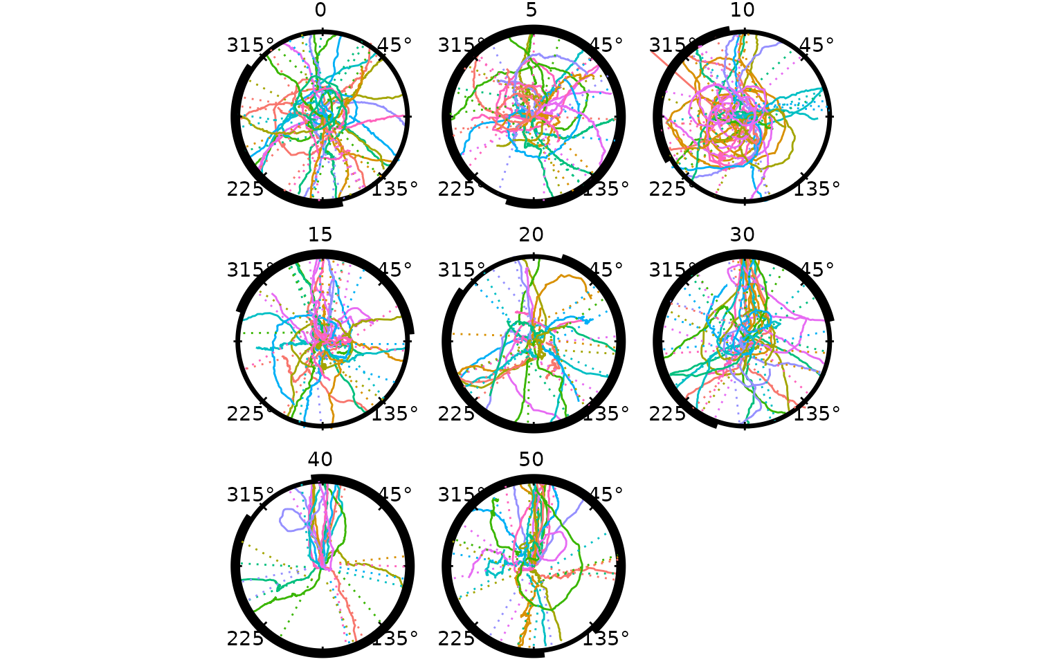

+ Heading points on top of the CI arc:

p <- p + add_heading_points(hd_cc, size = 4)
p
#> Warning: Removed 105 rows containing missing values or values outside the scale range
#> (`geom_path()`).
#> Warning: Removed 25 rows containing missing values or values outside the scale range
#> (`geom_segment()`).
#> Warning: Removed 25 rows containing missing values or values outside the scale range
#> (`geom_point()`).

p <- p + add_heading_arrow(hd_cc, colour_col = "arc", colour = "black")
p
#> Warning: Removed 105 rows containing missing values or values outside the scale range
#> (`geom_path()`).
#> Warning: Removed 25 rows containing missing values or values outside the scale range
#> (`geom_segment()`).
#> Warning: Removed 25 rows containing missing values or values outside the scale range
#> (`geom_point()`).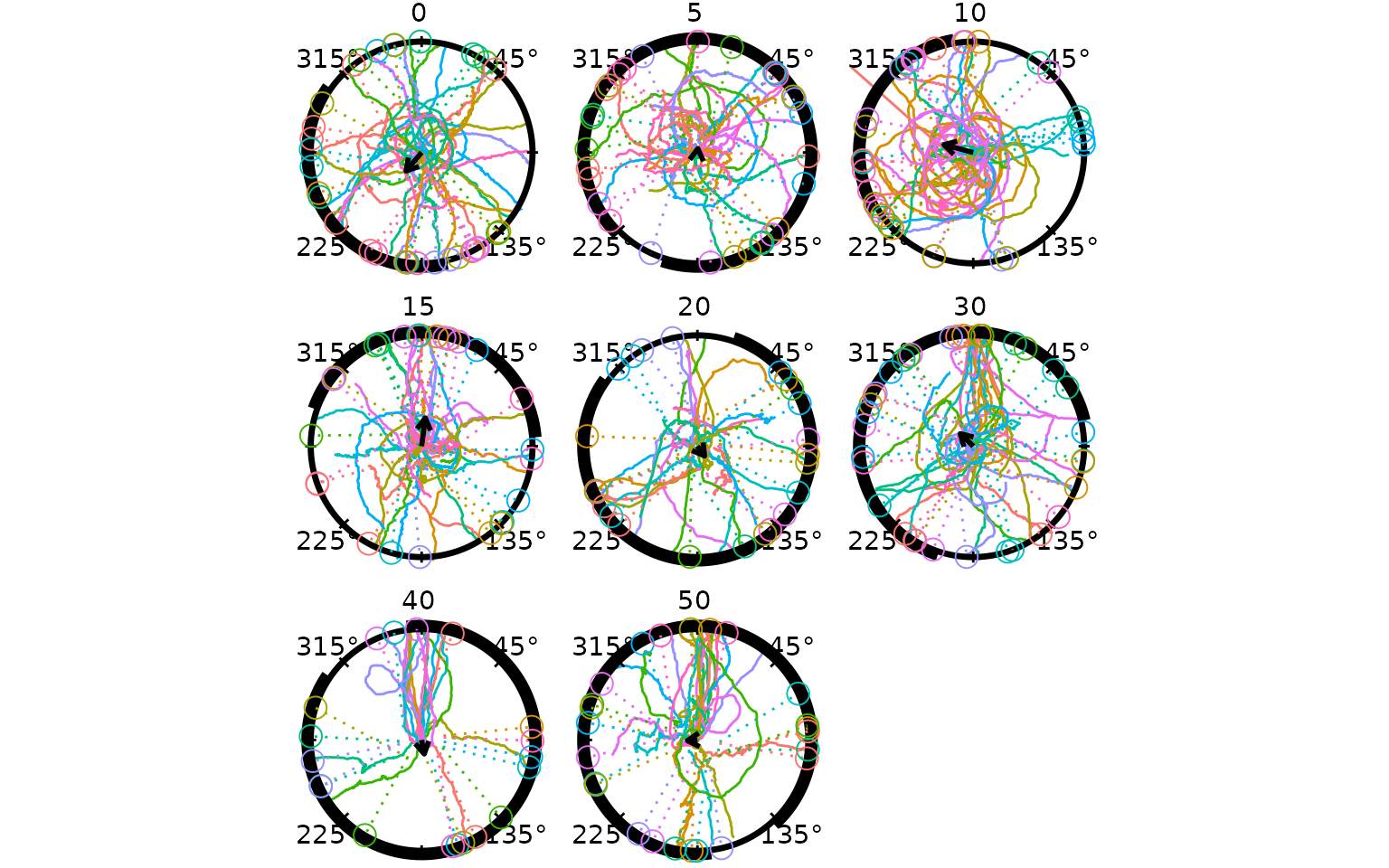

Each panel shows trajectories and heading markers coloured by per-trajectory cycling palette, a bootstrap CI arc at radius 1.05 in the condition colour (rendered behind the heading points), a solid mean direction arrow, and degree labels. All in clock convention (0° = toward reference, clockwise). Use strip_position = "inside" to place the label inside the plot area, or strip_labels = FALSE to suppress it.

Circular Density Overlays

Three functions handle directional density overlays; they are designed to compose cleanly with any density source:

Function	Role
compute_circular_density()	Estimates density from raw headings; returns a plain data frame of (theta, density) pairs
add_circular_density()	Renders any (theta, density) data frame as a radial overlay — agnostic to how the density was produced
add_heading_density()	Convenience wrapper: calls the two above in sequence

Three built-in methods are available in compute_circular_density(): "vonmises" (MLE via circular::mle.vonmises()), "kernel" (circular KDE), and "histogram" (bin counts). Because the computation and rendering steps are separate, the density column can be replaced with values from any other model — including a Bayesian posterior predictive density from brms — before calling add_circular_density():

dens_df <- compute_circular_density(hd, colour_col = "arc", method = "vonmises")
# replace with Bayesian posterior: dens_df$density <- my_brms_fitted_density(dens_df$theta)
add_circular_density(dens_df, colour_col = "arc", fill = "grey80", alpha = 0.35)

The convenience wrapper add_heading_density() skips the intermediate step when no substitution is needed. The combined panel plot below uses it to shade a per-condition von Mises density alongside the heading vectors:

radiate(cpunctatus_cc,
        group_col    = "trial_id",
        colour_col   = "cycle_colour",
        facets     = "arc",
        ncol         = 3,
        show_labels  = FALSE,
        show_arrow   = FALSE,
        display      = circ_display(zero = 0)) +
  add_heading_density(hd_cc, colour_col = "arc",
                      method = "vonmises", scale = 0.4,
                      fill = "grey80", alpha = 0.35) +
  add_heading_vectors(hd_cc) +
  add_heading_arrow(hd_cc, colour_col = "arc", colour = "black")
#> Warning: Removed 105 rows containing missing values or values outside the scale range
#> (`geom_path()`).
#> Warning: Removed 25 rows containing missing values or values outside the scale range
#> (`geom_segment()`).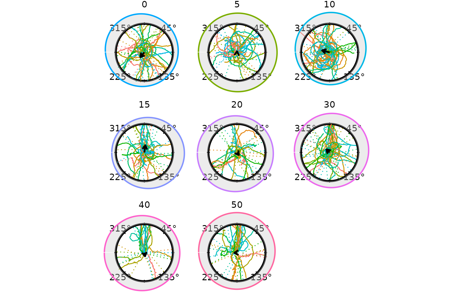

The shaded region is the von Mises density fitted to the crossing headings within each arc condition. A narrower, taller peak indicates more concentrated directional responses. Switch to method = "kernel" for a non-parametric estimate, or method = "histogram" for a raw count display.

Bootstrap Confidence Band

compute_circular_density() with boot_reps > 0 runs a non-parametric bootstrap: heading samples are drawn with replacement, a von Mises MLE is fitted to each replicate, and the density is re-evaluated on the same angular grid. The boot_alpha / 2 and 1 - boot_alpha / 2 quantiles across replicates become density_lower and density_upper columns, which add_circular_density() renders as a shaded band around the fitted curve.

dens_boot <- compute_circular_density(hd, colour_col = "arc",
                                      method = "vonmises",
                                      boot_reps = 499L, boot_alpha = 0.05,
                                      n_theta = 300L)

radiate(cpunctatus,
        group_col    = "trial_id",
        colour_cycle = 10,
        facets     = "arc",
        ncol         = 3,
        show_labels  = FALSE,
        show_arrow   = FALSE,
        display      = circ_display(zero = 0)) +
  add_circular_density(dens_boot, colour_col = "arc",
                       scale = 0.4, fill = "grey80", alpha = 0.35,
                       ci_fill = "grey60", ci_alpha = 0.35) +
  add_heading_arrow(hd, colour_col = "arc", colour = "black")
#> Warning: Removed 105 rows containing missing values or values outside the scale range
#> (`geom_path()`).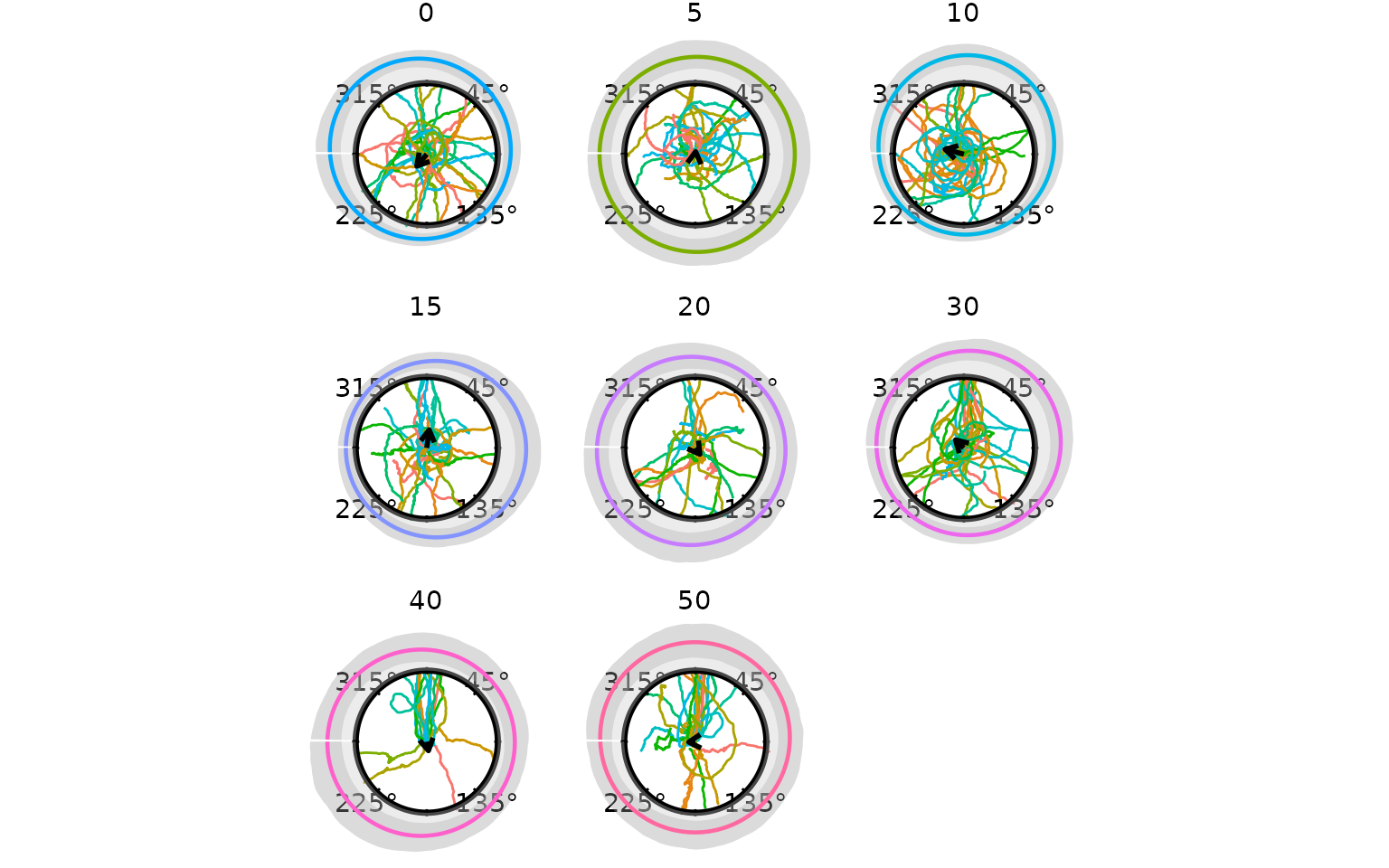

The darker band is the 95% bootstrap confidence interval for the fitted von Mises density. A wider band reflects greater parametric uncertainty, typically seen in the smaller or more diffuse conditions. The density_lower and density_upper columns in dens_boot can be replaced with interval values from a Bayesian model (e.g. the 2.5th and 97.5th percentiles of a brms posterior predictive distribution) before passing to add_circular_density().

Circular Summary Statistics

compute_circ_mean() returns the per-condition statistics behind the arrows above:

compute_circ_mean(hd, group_col = "arc")[, c("arc", "mean_dir", "resultant_R")]
#>   arc  mean_dir resultant_R
#> 1  10 1.3122762  0.27298867
#> 2  15 6.1535219  0.25745294
#> 3  20 3.7683984  0.10968390
#> 4  30 0.8051961  0.16285026
#> 5  40 3.3258479  0.12904693
#> 6   5 6.1710354  0.03518184
#> 7  50 1.6405047  0.09148952
#> 8   0 2.4441971  0.21852376

For within-trial path consistency (tortuosity), circ_summary() operates on the step-by-step angle distribution:

circ_summary(ts_demo)
#>           id   n t_start t_end   mean_dir resultant_R        kappa
#> 1     10_1_1  81       1    81 0.11601277  0.83986765    3.4526947
#> 2    10_10_1 299       1   299 2.27816423  0.15483083    0.3134475
#> 3    10_11_1  65      14    78 0.25433201  0.66719920    1.8194711
#> 4    10_12_1  48       2    49 2.30699848  0.90377927    5.4856988
#> 5    10_13_1  80      22   101 0.96510683  0.53748429    1.2768013
#> 6    10_14_1  30       1    30 4.76335993  0.97186701   18.0335307
#> 7    10_15_1  54       2    55 3.52077381  0.93703586    8.2159697
#> 8    10_16_1  78       2    79 3.07994139  0.75350741    2.3918496
#> 9    10_17_1  47       1    47 3.57548520  0.96788712   15.8324553
#> 10   10_19_1 282      18   299 1.95265552  0.37352800    0.8052313
#> 11    10_2_1  48       1    48 2.38407618  0.92287205    6.7636864
#> 12   10_20_1 257      35   291 3.28735826  0.06865973    0.1376444
#> 13   10_23_1 285      15   299 3.17651959  0.95049488   10.3693399
#> 14   10_24_1 299       1   299 4.41001073  0.99114749   56.7344981
#> 15   10_26_1 297       3   299 0.56922008  0.98833710   43.1254125
#> 16   10_27_1 287      13   299 1.27801742  0.17608487    0.3577705
#> 17   10_28_1  70       1    70 0.24722515  0.99017916   51.1658663
#> 18   10_29_1 160      33   192 5.88168170  0.89922506    5.2529045
#> 19    10_3_1 113       1   113 2.82658773  0.36596253    0.7864081
#> 20   10_33_1 292       8   299 2.63078292  0.99680196  156.5968961
#> 21   10_35_1 285      15   299 3.71725585  0.98345748   30.4814385
#> 22   10_39_1 209       8   216 1.74020125  0.87543282    4.3162149
#> 23   10_41_1 246      54   299 4.40674054  0.66683690    1.8175624
#> 24   10_45_1 297       3   299 1.94073553  0.96305715   13.7987172
#> 25    10_5_1  60       2    61 1.94603101  0.71894766    2.1293014
#> 26    10_6_1  91       1    91 5.38407117  0.73923539    2.2765340
#> 27    10_7_1  56       1    56 3.03029422  0.81454694    3.0508663
#> 28    10_8_1  87       1    87 0.28440324  0.98625686   36.6370102
#> 29    10_9_1 299       1   299 1.28909699  0.44454476    0.9914081
#> 30   15_10_1 299       1   299 2.55980784  0.94235363    8.9462985
#> 31   15_11_1 299       1   299 6.22819541  0.99982898 2923.9000317
#> 32   15_13_1  86       1    86 2.34142569  0.97038308   17.1436340
#> 33   15_14_1 299       1   299 4.50120997  0.96268696   13.6645884
#> 34   15_16_1 299       1   299 2.22838041  0.05176624    0.1036715
#> 35   15_19_1 136       1   136 1.49830203  0.97451676   19.8805068
#> 36    15_2_1 298       2   299 3.78567731  0.56143361    1.3608600
#> 37   15_21_1 299       1   299 0.30348015  0.99696169  164.8165327
#> 38   15_23_1 299       1   299 5.46169359  0.50809640    1.1755835
#> 39   15_24_1 299       1   299 6.01136043  0.99737845  190.9775615
#> 40   15_25_1 201      15   215 3.49231678  0.24577237    0.5071377
#> 41   15_26_1 180       4   183 4.59130526  0.99325588   74.3912426
#> 42   15_27_1 299       1   299 3.27544567  0.51244674    1.1889113
#> 43   15_28_1 205       1   205 2.51823083  0.94955008   10.1805789
#> 44   15_29_1 181       1   181 1.40296402  0.30838298    0.6484174
#> 45    15_3_1 263      20   282 4.14828843  0.90299967    5.4442830
#> 46   15_30_1 280       1   280 2.98748265  0.99798753  248.7010630
#> 47   15_32_1 299       1   299 5.96415656  0.98966372   48.6271972
#> 48   15_35_1 233       1   233 0.20853032  0.78788735    2.7223881
#> 49   15_36_1 299       1   299 2.77136926  0.47808052    1.0862441
#> 50   15_41_1 192       6   197 0.45932573  0.94218791    8.9215039
#> 51   15_42_1  92       1    92 3.50831648  0.97564825   20.7917310
#> 52   15_44_1 225       7   231 3.10874826  0.32496901    0.6872765
#> 53   15_47_1 225       1   225 0.17240450  0.99548491  110.9914309
#> 54   15_48_1 225       1   225 0.18326845  0.99518116  104.0112534
#> 55   15_49_1 299       1   299 1.67764329  0.99937551  800.9029328
#> 56   15_50_1 299       1   299 1.07588619  0.42856981    0.9479043
#> 57   15_51_1 181       1   181 6.13306449  0.99791415  239.9614134
#> 58    15_7_1 175       3   177 0.24885314  0.98512977   33.8798784
#> 59    15_9_1 279       3   281 5.14054126  0.72395950    2.1640461
#> 60   20_10_1 299       1   299 3.90847302  0.95728614   11.9724167
#> 61   20_11_1 284       8   291 5.65755647  0.77852741    2.6237026
#> 62   20_13_1 287       2   288 4.01880340  0.62800624    1.6288621
#> 63   20_14_1 135       1   135 0.25507384  0.97496332   20.2302890
#> 64   20_16_1 216       8   223 5.39642116  0.92479381    6.9285163
#> 65   20_18_1 283       2   284 5.04291139  0.71006271    2.0700665
#> 66   20_19_1  78      21    98 1.79807786  0.97876779   23.8072301
#> 67    20_2_1 227       1   227 1.51703975  0.89133744    4.8963315
#> 68   20_20_1  85       1    85 2.68502012  0.75287781    2.3865301
#> 69   20_22_1 299       1   299 0.18918312  0.97859808   23.6205660
#> 70   20_24_1 299       1   299 4.19233539  0.97193537   18.0767966
#> 71   20_26_1 274       7   280 3.01169447  0.50723092    1.1729438
#> 72   20_27_1  84      10    93 2.90554888  0.65560451    1.7598548
#> 73   20_28_1 246       5   250 2.64039413  0.94119258    8.7755355
#> 74   20_29_1  41      59    99 0.92989363  0.95902177   12.4675179
#> 75    20_3_1 241      43   283 4.13256041  0.62193439    1.6018575
#> 76   20_30_1 299       1   299 4.06111336  0.99762883  211.1168970
#> 77   20_33_1 105      40   144 0.42291825  0.95171682   10.6244482
#> 78   20_35_1 299       1   299 0.06807526  0.99863680  367.0353916
#> 79   20_36_1 274       1   274 0.95650996  0.51392567    1.1934650
#> 80   20_39_1  71      81   151 2.29183469  0.93249560    7.6837756
#> 81   20_41_1 202      50   251 6.19127720  0.96381695   14.0826192
#> 82   20_47_1 120      62   181 5.04036796  0.31089917    0.6542699
#> 83   20_48_1 110      16   125 3.55333429  0.91803621    6.3832960
#> 84    20_5_1 269      31   299 0.51898415  0.92700037    7.1285334
#> 85    20_7_1 297       3   299 2.59039500  0.94274263    9.0050647
#> 86    20_9_1 299       1   299 5.16322703  0.99372483   79.9314711
#> 87    30_1_1  73      20    92 3.39275362  0.90071602    5.3267432
#> 88   30_10_1  38       1    38 6.07733907  0.99087223   55.0313608
#> 89   30_11_1  60       1    60 4.20293090  0.93157618    7.5846364
#> 90   30_12_1  52       7    58 3.29319603  0.96586000   14.9087581
#> 91   30_13_1  50      35    84 4.62774407  0.93530935    8.0047587
#> 92   30_14_1  34       1    34 2.06777042  0.99308649   72.5747768
#> 93   30_15_1  41       1    41 6.13222047  0.98975264   49.0469529
#> 94   30_16_1  50       1    50 4.01534137  0.94753425    9.8006137
#> 95   30_17_1  51       1    51 5.36276056  0.89836243    5.2111831
#> 96   30_18_1 284      16   299 2.28433577  0.99345023   76.5909878
#> 97   30_19_1  71      16    86 2.73210591  0.90590373    5.6020747
#> 98    30_2_1  73      12    84 5.47578231  0.39447530    0.8582953
#> 99   30_20_1 129       6   134 1.77295330  0.40866735    0.8950846
#> 100  30_24_1 299       1   299 5.43793062  0.99482668   96.9017712
#> 101  30_26_1 177       1   177 3.40104741  0.96939648   16.5997696
#> 102  30_27_1 216      27   242 5.61946327  0.67400152    1.8558867
#> 103  30_28_1 139      19   157 0.03150473  0.97900913   24.0778975
#> 104  30_29_1 200      53   252 3.00899101  0.96466914   14.4155908
#> 105   30_3_1  56       7    62 4.99839006  0.70272866    2.0232828
#> 106  30_30_1 178       1   178 0.38647092  0.98072191   26.1935262
#> 107  30_32_1 182      72   253 0.03134930  0.81603080    3.0716307
#> 108  30_33_1 138      13   150 6.02909798  0.97977956   24.9851666
#> 109  30_36_1 299       1   299 4.44004481  0.99022264   51.3922525
#> 110  30_39_1 199      44   242 0.72661645  0.90772186    5.7059632
#> 111  30_42_1  58       1    58 2.05768991  0.99873914  396.8056248
#> 112  30_43_1 241      50   290 2.16904391  0.98470451   32.9451828
#> 113  30_44_1 169      26   194 0.64805093  0.73352021    2.2332239
#> 114  30_46_1 273      27   299 2.18430623  0.63729476    1.6713754
#> 115  30_47_1 288      12   299 4.94467482  0.62368005    1.6095600
#> 116  30_49_1 294       6   299 2.20328778  0.87515734    4.3074881
#> 117   30_5_1  53       1    53 5.61673329  0.81208153    3.0170197
#> 118  30_50_1  65       1    65 5.81959476  0.96142054   13.2252189
#> 119  30_51_1 205       9   213 3.44708860  0.05506557    0.1102985
#> 120   30_6_1  48       6    53 5.83079548  0.98006564   25.3399272
#> 121   30_7_1  39       1    39 2.32792086  0.96191934   13.3947788
#> 122   30_8_1 129       1   129 0.68981333  0.35496752    0.7593580
#> 123   30_9_1  90       4    93 6.16244951  0.64077539    1.6877004
#> 124  40_10_1 133      10   142 6.00447436  0.40888368    0.8956509
#> 125  40_11_1 299       1   299 6.11919465  0.99801351  251.9504713
#> 126  40_13_1 191       2   192 5.59272404  0.36390208    0.7813117
#> 127  40_14_1 259       7   265 2.43980261  0.85412471    3.7401799
#> 128  40_16_1 221      31   251 1.98421263  0.95133761   10.5439058
#> 129  40_17_1 104       2   105 6.16532152  0.88894377    4.7982510
#> 130  40_18_1 116     145   260 0.79804169  0.72171201    2.1483416
#> 131  40_19_1  90       9    98 0.26186201  0.98727821   39.5574662
#> 132   40_2_1 118      12   129 6.12041950  0.77375815    2.5761448
#> 133  40_24_1 205       2   206 1.04904279  0.87601778    4.3348772
#> 134  40_26_1 135      10   144 3.71903067  0.80816710    2.9648865
#> 135  40_27_1 138       3   140 0.56835462  0.71555686    2.1063497
#> 136   40_3_1 124      28   151 0.17927597  0.78604298    2.7023492
#> 137  40_30_1  99       3   101 5.81357489  0.96389623   14.1129341
#> 138  40_32_1  96     128   223 0.08177663  0.67625013    1.8681736
#> 139  40_33_1 126       3   128 0.46419774  0.80410230    2.9127254
#> 140  40_49_1  46       2    47 6.17303314  0.99806524  258.6813066
#> 141   40_5_1  94       4    97 0.18349674  0.89185689    4.9181965
#> 142   40_6_1 277       4   280 6.20636421  0.57290195    1.4031283
#> 143   40_7_1 264      36   299 0.10986755  0.99581738  119.7939241
#> 144   5_10_1 201       3   203 1.32889449  0.89693381    5.1436384
#> 145   5_11_1 298       2   299 3.18129611  0.59089708    1.4724272
#> 146   5_12_1 158       2   159 0.39855843  0.94047525    8.6733731
#> 147   5_13_1 191       6   196 0.39832703  0.73418987    2.2382200
#> 148   5_16_1 208       1   208 3.56967734  0.93046175    7.4679993
#> 149   5_17_1 142       1   142 5.65665650  0.99938804  817.2909887
#> 150   5_19_1 208       1   208 1.51114689  0.97325096   18.9525174
#> 151    5_2_1 137     163   299 0.22200488  0.91587458    6.2274880
#> 152   5_21_1 260       1   260 5.07208979  0.98465297   32.8354153
#> 153   5_22_1 297       3   299 0.29515255  0.61239287    1.5605968
#> 154   5_23_1 299       1   299 5.68981823  0.99585195  120.7900770
#> 155   5_25_1 280      20   299 3.93085155  0.39653127    0.8635816
#> 156   5_26_1 296       3   298 6.24589318  0.93833171    8.3822940
#> 157   5_29_1 184       1   184 6.05913072  0.40361072    0.8818958
#> 158    5_3_1 261       2   262 3.82717578  0.79910149    2.8511352
#> 159   5_32_1 299       1   299 2.21265215  0.99370379   79.6651959
#> 160   5_35_1 299       1   299 5.71977087  0.99512318  102.7776372
#> 161   5_36_1 299       1   299 2.27394875  0.98980596   49.3021177
#> 162   5_41_1 105       1   105 5.31642185  0.98211878   28.2191104
#> 163   5_42_1 191       1   191 6.06074139  0.28949964    0.6049568
#> 164   5_44_1 299       1   299 5.98267984  0.94016727    8.6302640
#> 165   5_45_1 299       1   299 5.53354052  0.99502366  100.7273688
#> 166   5_46_1 299       1   299 3.06873896  0.85861001    3.8467114
#> 167   5_47_1 149       1   149 5.96766840  0.95295904   10.8974036
#> 168   5_48_1 274       1   274 3.09024609  0.97820154   23.1957256
#> 169   5_49_1 299       1   299 1.14779301  0.94104956    8.7549686
#> 170    5_5_1 269      31   299 3.51190462  0.31626160    0.6667928
#> 171    5_6_1 256      44   299 0.12235832  0.85720948    3.8127114
#> 172    5_7_1 215       1   215 4.77971702  0.89910205    5.2469113
#> 173    5_8_1 123       1   123 4.22910498  0.98116197   26.7992248
#> 174    5_9_1 299       1   299 1.15330738  0.68674076    1.9272347
#> 175   50_1_1  65       1    65 6.19771559  0.99913654  579.3173742
#> 176  50_10_1 194       4   197 2.28619987  0.87947832    4.4490468
#> 177  50_11_1 256       2   257 6.25526767  0.34406464    0.7328779
#> 178  50_14_1 132       2   133 6.03483957  0.98049111   25.8867811
#> 179  50_16_1 298       2   299 6.25805730  0.88495925    4.6441505
#> 180   50_2_1  62      11    72 3.21592025  0.98097149   26.5336128
#> 181  50_20_1 155      73   227 0.73455550  0.92704569    7.1327691
#> 182  50_22_1  77      54   130 0.34123154  0.98576413   35.3779399
#> 183  50_24_1 282      18   299 1.45208632  0.96835103   16.0604962
#> 184  50_25_1 123      37   159 5.75907144  0.96936065   16.5806790
#> 185  50_26_1 124      19   142 4.35624530  0.94413496    9.2221296
#> 186  50_27_1 130       1   130 3.08946442  0.99090064   55.2023782
#> 187  50_28_1 229      11   239 3.45828698  0.98948172   47.7902484
#> 188  50_29_1 299       1   299 0.66366149  0.98645976   37.1821034
#> 189   50_3_1 125       1   125 0.15990034  0.95491684   11.3581900
#> 190  50_32_1 288      12   299 1.53825754  0.98379715   31.1149208
#> 191  50_33_1 261       1   261 6.05266750  0.99283917   70.0769783
#> 192  50_39_1  59       6    64 5.63262124  0.99709946  172.6330222
#> 193  50_40_1 133       3   135 5.97765964  0.85551295    3.7724289
#> 194  50_41_1 103      38   140 0.92126074  0.58873647    1.4639020
#> 195  50_42_1 107      59   165 6.18312554  0.99447837   90.8049876
#> 196  50_43_1 102       2   103 6.23777013  0.99124588   57.3692725
#> 197  50_44_1 203      35   237 0.26364345  0.97867479   23.7045728
#> 198  50_50_1 179       6   184 4.90491763  0.08519778    0.1710177
#> 199   50_7_1 299       1   299 6.26336680  0.99001778   50.3428105
#> 200   50_9_1  90       1    90 0.36394343  0.92791231    7.2147925
#> 201  con_1_1 147       1   147 1.29473659  0.98007630   25.3533361
#> 202 con_10_1 120       8   127 3.47730318  0.90937123    5.8038446
#> 203 con_11_1 118       1   118 5.25384538  0.95278182   10.8575831
#> 204 con_12_1 129      45   173 0.38534017  0.92386876    6.8481303
#> 205 con_13_1 149       1   149 4.24942089  0.97254953   18.4751632
#> 206 con_14_1 155      52   206 1.77863176  0.87041196    4.1630788
#> 207 con_15_1 118       1   118 4.38496821  0.98996964   50.1024458
#> 208 con_16_1 221       6   226 5.20647224  0.84991454    3.6464155
#> 209 con_19_1 266      34   299 5.01384177  0.27536779    0.5729354
#> 210  con_2_1 136      24   159 4.37473303  0.91887910    6.4463154
#> 211 con_20_1 299       1   299 1.69562541  0.37926374    0.8196204
#> 212 con_23_1 115       2   116 3.73039640  0.79732483    2.8299030
#> 213 con_24_1 291       1   291 5.38453689  0.99489603   98.2149372
#> 214 con_25_1 142       1   142 2.26654959  0.96467020   14.4160144
#> 215 con_26_1 277       2   278 3.37470337  0.99053493   53.0793738
#> 216 con_27_1 110       4   113 0.04989460  0.79092220    2.7560325
#> 217 con_28_1 256       3   258 0.36443605  0.20171194    0.4119093
#> 218 con_29_1 290       1   290 2.80214800  0.87108892    4.1830180
#> 219  con_3_1 130      43   172 0.27829493  0.98783410   41.3530841
#> 220 con_33_1  45       1    45 2.09379998  0.99253604   67.2414025
#> 221 con_35_1 294       3   296 5.55192506  0.97266365   18.5511572
#> 222 con_36_1 299       1   299 5.19699304  0.95996382   12.7542429
#> 223 con_39_1 128       9   136 4.22334572  0.99369898   79.6045452
#> 224 con_41_1 137      10   146 5.64130692  0.74099920    2.2902154
#> 225 con_44_1 136       1   136 3.44949153  0.79236089    2.7722824
#> 226 con_47_1 281      19   299 1.04005905  0.19074572    0.3886419
#> 227 con_48_1 164      32   195 5.76965270  0.59891339    1.5045773
#> 228 con_49_1 299       1   299 0.11174903  0.99885384  436.4888558
#> 229  con_5_1 109       2   110 1.96347912  0.97036793   17.1350039
#> 230 con_50_1 299       1   299 3.56823469  0.19359006    0.3946619
#> 231 con_51_1 196      11   206 3.64874010  0.99212806   63.7697499
#> 232  con_6_1 114       1   114 3.04482025  0.99546073  110.4015185
#> 233  con_7_1 134      19   152 2.11124516  0.87734213    4.3777969
#> 234  con_8_1 213      68   280 0.81824501  0.98924503   46.7441973
#> 235  con_9_1 299       1   299 6.20059653  0.33178954    0.7034546

High resultant lengths (close to 1) indicate very consistent step directions within a trial.

Alternative Heading Rules

derive_headings() supports fourteen built-in rules. "crossing" is well suited to echinoderm-style tracks — moderate tortuosity, consistent outward movement — but other rules may be more appropriate depending on the taxon and experimental design. Use list_heading_rules() to see all available names; custom rules can be added with register_heading_rule().

Two parameter-free alternatives are especially useful:

Rule	What it returns	Typical use
"distal"	Angular position of the frame with the largest radius	Straight outward paths (dung beetles, ballistic homing)
"net"	Direction of the start-to-end displacement vector	Sinuous or multi-phase paths where only net displacement matters

distal

The distal rule takes atan2(y, x) at the frame where the subject is farthest from the centre. It requires no ring parameters and never returns NA because every trial has a most-distal frame.

hd_distal <- derive_headings(cpunctatus, rule = "distal",
                              return_coords = TRUE)
names(hd_distal)[names(hd_distal) == "id"] <- "trial_id"
# join the target half-width (arc) from the dataset, as for the crossing rule
hd_distal     <- merge(hd_distal, arc_map, by = "trial_id")
hd_distal$arc <- factor(hd_distal$arc)
attr(hd_distal, "display") <- circ_display(zero = 0)

Per-condition resultant lengths from "distal" are very close to those from "crossing", consistent with millipede tracks being fairly direct:

sm_cross  <- compute_circ_mean(hd,       group_col = "arc")[, c("arc", "resultant_R")]
sm_distal <- compute_circ_mean(hd_distal, group_col = "arc")[, c("arc", "resultant_R")]
names(sm_cross)[2]  <- "crossing"
names(sm_distal)[2] <- "distal"
merge(sm_cross, sm_distal, by = "arc")
#>   arc   crossing     distal
#> 1   0 0.21852376 0.23531457
#> 2  10 0.27298867 0.07055967
#> 3  15 0.25745294 0.24477975
#> 4  20 0.10968390 0.07326231
#> 5  30 0.16285026 0.12936762
#> 6  40 0.12904693 0.06536414
#> 7   5 0.03518184 0.07181952
#> 8  50 0.09148952 0.15790182

Visualising the distal headings on the per-condition panel confirms that the spatial pattern is consistent with the crossing method:

cpunctatus_cc_d        <- cpunctatus
cpunctatus_cc_d@data   <- assign_cycle_colours(cpunctatus@data,
                                              id_col    = "trial_id",
                                              n         = 10,
                                              panel_col = "arc")
colour_map_d <- unique(cpunctatus_cc_d@data[, c("trial_id", "cycle_colour")])
hd_distal_cc <- merge(hd_distal, colour_map_d, by = "trial_id", all.x = TRUE)
attr(hd_distal_cc, "display")    <- attr(hd_distal, "display", exact = TRUE)
attr(hd_distal_cc, "colour_col") <- "cycle_colour"

radiate(cpunctatus_cc_d,
        group_col   = "trial_id",
        colour_col  = "cycle_colour",
        facets    = "arc",
        ncol        = 3,
        show_labels = FALSE,
        show_arrow  = FALSE,
        display     = circ_display(zero = 0)) +
  add_heading_interval(hd_distal_cc, group_col = "arc", colour = "black",
                       stat = "bootstrap_ci", boot_reps = 999L) +
  add_heading_points(hd_distal_cc, size = 4) +
  add_heading_arrow(hd_distal_cc, colour_col = "arc", colour = "black")
#> Warning: Removed 105 rows containing missing values or values outside the scale range
#> (`geom_path()`).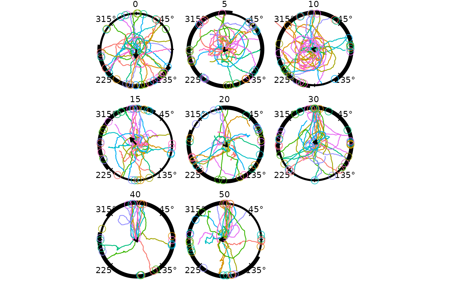

Because millipede tracks are nearly radial, the heading estimates agree closely across methods. For more sinuous species (moths, pigeons) the choice of rule has a larger influence on the result.

net

The net rule returns the direction of the vector from the first recorded position to the last, ignoring all intermediate points. It is the fastest possible estimate and is the natural match for GPS vanishing-bearing studies where only the release and final observed positions are available.

hd_net <- derive_headings(cpunctatus, rule = "net")
names(hd_net)[names(hd_net) == "id"] <- "trial_id"
# join the target half-width (arc) from the dataset, as for the crossing rule
hd_net     <- merge(hd_net, arc_map, by = "trial_id")
hd_net$arc <- factor(hd_net$arc)

sm_net <- compute_circ_mean(hd_net, group_col = "arc")[, c("arc", "resultant_R")]
names(sm_net)[2] <- "net"
Reduce(function(a, b) merge(a, b, by = "arc"),
       list(sm_cross, sm_distal, sm_net))
#>   arc   crossing     distal        net
#> 1   0 0.21852376 0.23531457 0.22962978
#> 2  10 0.27298867 0.07055967 0.05152922
#> 3  15 0.25745294 0.24477975 0.23894631
#> 4  20 0.10968390 0.07326231 0.02827464
#> 5  30 0.16285026 0.12936762 0.11498421
#> 6  40 0.12904693 0.06536414 0.06850022
#> 7   5 0.03518184 0.07181952 0.05236747
#> 8  50 0.09148952 0.15790182 0.15353222

For these tracks the three methods give very similar resultant lengths. Larger differences would be expected for species with complex search behaviour before committing to a direction.