Circular Statistics and Distribution Overlays • radiatR

if (requireNamespace("pkgload", quietly = TRUE)) {
  pkgload::load_all("..", export_all = FALSE, helpers = FALSE, quiet = TRUE)
} else if (requireNamespace("radiatR", quietly = TRUE)) {
  library(radiatR)
} else {
  stop("Package 'radiatR' not installed and 'pkgload' not available.")
}
library(ggplot2)

Overview

The main radiatR vignette covers the path from raw tracking files to a plotted set of headings. This vignette picks up from a heading data frame and shows the analysis layer:

Dispersion summaries — circ_dispersion(), sector_summary()
Parametric fits — vonmises_fit(), wrappedcauchy_fit()
Hypothesis tests — test_uniformity(), test_mean_directions(), test_concentration(), all with multiple-comparison correction
Correlation — circ_cor() (circular-linear and circular-circular)
Distribution overlays — add_angle_rose(), add_vonmises_density(), add_wrappedcauchy_density(), add_circular_kde()
Significance geometry — add_critical_r() (Rayleigh / V-test circle) and add_critical_v_line() (V-test boundary)

Every statistics function takes a data frame with a heading column in radians (default name "heading") and returns a tidy data frame, so the results drop straight into dplyr, knitr::kable(), or further plotting.

A heading data frame

We derive one heading per trial from the bundled cpunctatus dataset with the ring-crossing rule, then attach each trial’s target half-width (arc) for grouping. This is the same construction used in the main vignette.

data(cpunctatus)

hd <- derive_headings(cpunctatus, rule = "crossing",
                      circ0 = 0.2, circ1 = 0.4,
                      coords = "relative",
                      angle_convention = "clock")
names(hd)[names(hd) == "id"] <- "trial_id"

# attach target half-width (arc) from the dataset, by trial
arc_map  <- unique(cpunctatus@data[, c("trial_id", "arc")])
hd       <- merge(hd, arc_map, by = "trial_id")
hd$arc   <- factor(hd$arc)

# keep trials with a defined crossing heading
hd <- hd[is.finite(hd$heading), , drop = FALSE]
head(hd[, c("trial_id", "arc", "heading")])
#>   trial_id arc   heading
#> 1   10_1_1  10 0.2777794
#> 2  10_10_1  10 3.0376774
#> 3  10_11_1  10 6.0710737
#> 4  10_12_1  10 2.2074837
#> 5  10_13_1  10 0.9322361
#> 6  10_14_1  10 4.7955587

The heading column is in radians, reference-relative (0 = toward the target). Everything below operates on that column.

Dispersion summaries

circ_dispersion() returns the mean direction, resultant length R, and circular standard deviation. Grouping by arc gives one row per condition.

circ_dispersion(hd, group_col = "arc")
#>   arc     mean_dir resultant_R   circ_sd  n
#> 1  10  1.980062802  0.25662879 1.6493178 35
#> 2  15  0.002875648  0.18589914 1.8344214 27
#> 3  20  2.960834000  0.07603959 2.2700225 24
#> 4  30 -0.453000259  0.06016175 2.3709570 34
#> 5  40  0.075648794  0.64058845 0.9437882 19
#> 6   5  0.394217868  0.17579270 1.8646446 30
#> 7  50 -0.173753450  0.44404605 1.2742268 24
#> 8   0  2.276557489  0.08000698 2.2475059 33

R runs from 0 (uniformly scattered) to 1 (all headings identical); the circular SD moves the opposite way. For dense per-frame heading series — gaze direction from a tethered animal, say — sector_summary() bins the angles and reports dwell proportions per sector:

sector_summary(hd, sectors = 8L)
#>        sector  mid_angle count proportion
#> 1 -158degrees -2.7488936    27 0.11946903
#> 2 -112degrees -1.9634954    18 0.07964602
#> 3  -68degrees -1.1780972    20 0.08849558
#> 4  -22degrees -0.3926991    42 0.18584071
#> 5   22degrees  0.3926991    45 0.19911504
#> 6   68degrees  1.1780972    13 0.05752212
#> 7  112degrees  1.9634954    35 0.15486726
#> 8  158degrees  2.7488936    26 0.11504425

Parametric fits

vonmises_fit() estimates the mean direction $\mu$ and concentration $\kappa$ by maximum likelihood, with asymptotic standard errors and a confidence interval on $\mu$ :

vonmises_fit(hd, group_col = "arc")[, c("arc", "mu_deg", "kappa", "n")]
#>   arc      mu_deg     kappa  n
#> 1  10 113.4492417 0.5310863 35
#> 2  15   0.1647625 0.3784077 27
#> 3  20 169.6432921 0.1525210 24
#> 4  30 -25.9550030 0.1205419 34
#> 5  40   4.3343566 1.6868180 19
#> 6   5  22.5870200 0.3571578 30
#> 7  50  -9.9553394 0.9900343 24
#> 8   0 130.4371359 0.1605288 33

wrappedcauchy_fit() is the heavier-tailed alternative — more robust when the data have outliers or weak directionality. Its concentration $\rho$ is bounded to $[0, 1)$ :

wrappedcauchy_fit(hd, group_col = "arc")[, c("arc", "mu_deg", "rho", "n")]
#>   arc     mu_deg        rho  n
#> 1  10 118.338958 0.25480084 35
#> 2  15   4.745037 0.27375349 27
#> 3  20 159.559101 0.09056095 24
#> 4  30 339.103222 0.08571126 34
#> 5  40   6.248322 0.75905693 19
#> 6   5  25.796263 0.15937039 30
#> 7  50 351.847489 0.68966189 24
#> 8   0 133.599471 0.08467292 33

Both return a row per group, so a quick merge() puts the two concentration estimates side by side for comparison.

Hypothesis tests

Uniformity

test_uniformity() asks, per group, whether the headings have any preferred direction. The Rayleigh test gives an exact p-value; when testing many conditions at once, pass p_adjust for a corrected p_value_adj column:

test_uniformity(hd, group_col = "arc", test = "rayleigh", p_adjust = "BH")
#>   arc  statistic     p_value  n     test p_value_adj
#> 1  10 0.25662879 0.099244958 35 rayleigh 0.264653222
#> 2  15 0.18589914 0.397036850 27 rayleigh 0.638463349
#> 3  20 0.07603959 0.872766166 24 rayleigh 0.885708681
#> 4  30 0.06016175 0.885708681 34 rayleigh 0.885708681
#> 5  40 0.64058845 0.000186684 19 rayleigh 0.001493472
#> 6   5 0.17579270 0.399039593 30 rayleigh 0.638463349
#> 7  50 0.44404605 0.007583494 24 rayleigh 0.030333977
#> 8   0 0.08000698 0.811900045 33 rayleigh 0.885708681

Equal mean directions

test_mean_directions() is the Watson-Williams test — the circular analogue of a one-way ANOVA on the mean angle. The omnibus form asks whether any group differs:

test_mean_directions(hd, group_col = "arc")
#>   n_groups statistic df1 df2     p_value            test
#> 1        8  8.230315   7 218 6.70879e-09 Watson-Williams

Set pairwise = TRUE for all pairwise comparisons; p_adjust is strongly recommended here because the number of comparisons grows quickly:

pw <- test_mean_directions(hd, group_col = "arc",
                           pairwise = TRUE, p_adjust = "holm")
head(pw[order(pw$p_value_adj), ])
#>    group1 group2 statistic df1 df2      p_value            test  p_value_adj
#> 14     20     30  68.71016   1  56 2.590906e-11 Watson-Williams 7.254536e-10
#> 22     30      0  45.35938   1  65 5.086470e-09 Watson-Williams 1.373347e-07
#> 6      10     50  31.92401   1  57 5.341214e-07 Watson-Williams 1.388716e-05
#> 4      10     40  24.34873   1  52 8.658990e-06 Watson-Williams 2.164747e-04
#> 1      10     15  16.68434   1  60 1.328071e-04 Watson-Williams 3.187369e-03
#> 13     15      0  16.32869   1  58 1.586887e-04 Watson-Williams 3.649841e-03

Equal concentrations

test_concentration() checks whether the groups are equally concentrated (the circular analogue of a test for equal variances), a key assumption behind the Watson-Williams test above:

test_concentration(hd, group_col = "arc")
#>   statistic df    p_value        test
#> 1  14.23259  7 0.04719587 equal.kappa

Circular correlation

circ_cor() measures the association between headings and a covariate. With x_type = "linear" (the default) it computes the circular-linear correlation — here, whether heading direction is associated with the numeric target half-width:

hd$arc_num <- as.numeric(as.character(hd$arc))
circ_cor(hd, x_col = "arc_num", angle_col = "heading", x_type = "linear")
#>           r   n            type statistic df    p_value
#> 1 0.2175965 226 circular-linear   10.7007  2 0.00474648

The returned r is unsigned (association strength, 0–1); the test statistic $n r^2$ is approximately $\chi^2_2$ . For two angular variables, pass x_type = "circular" to get Fisher’s $\rho \in [-1, 1]$ .

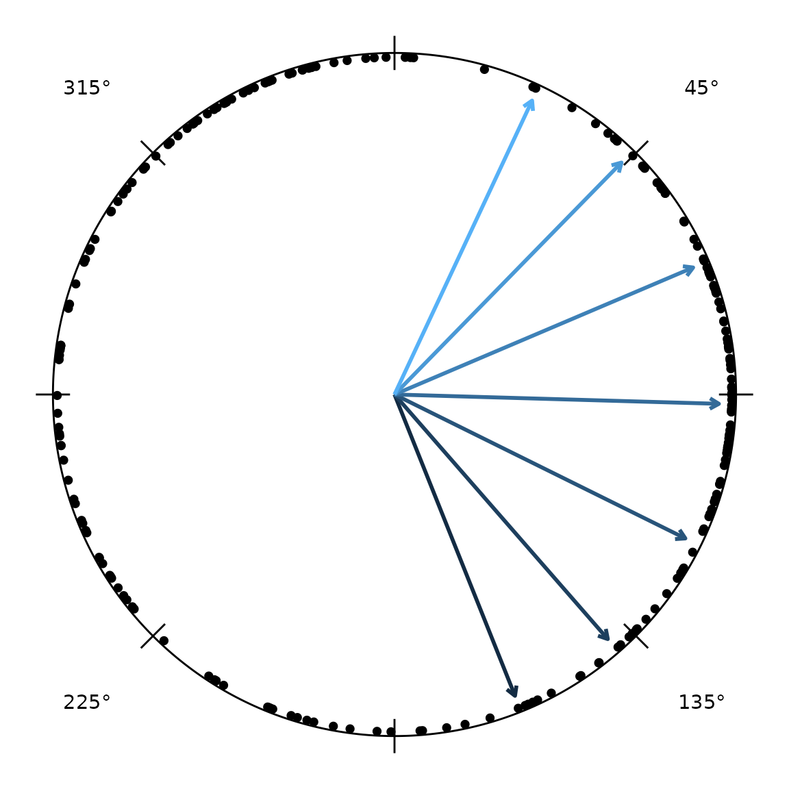
Distribution overlays

The overlay layers draw an angular distribution in the same Cartesian unit-disc space as radiate(), so they compose onto a bare circular canvas with +. We build that canvas once:

canvas <- ggplot() + coord_fixed() +
  add_circ(radius = 1) +
  theme_void()

A rose diagram bins the headings into wedges; the parametric and non-parametric density curves overlay on top. Giving every layer the same scale aligns their radii, so the shapes can be compared directly:

vm <- vonmises_fit(hd)        # pooled fit (group_col = NULL)
wc <- wrappedcauchy_fit(hd)

canvas +
  add_angle_rose(hd, bins = 12, scale = 0.8, fill = "grey80") +
  add_circular_kde(hd, scale = 0.8, colour = "tomato") +
  add_vonmises_density(vm, scale = 0.8, colour = "steelblue") +
  add_wrappedcauchy_density(wc, scale = 0.8, colour = "darkorange")

The grey wedges are the empirical rose; the steelblue curve is the von Mises fit, darkorange the wrapped Cauchy, and tomato a circular kernel density estimate. Where the parametric curves track the rose closely the fit is good; a systematic gap (especially in the tails) is the cue to prefer the heavier-tailed wrapped Cauchy.

Per-group overlays

Every overlay that summarises headings takes a colour_col, so a single call draws one element per group, coloured by it – handy for comparing conditions on one plot. Here the mean-direction arrow (add_heading_arrow()) and its bootstrap confidence interval (add_heading_interval()) are split by target half-width (arc):

canvas +
  add_heading_arrow(hd,    colour_col = "arc") +
  add_heading_interval(hd, colour_col = "arc", stat = "bootstrap_ci")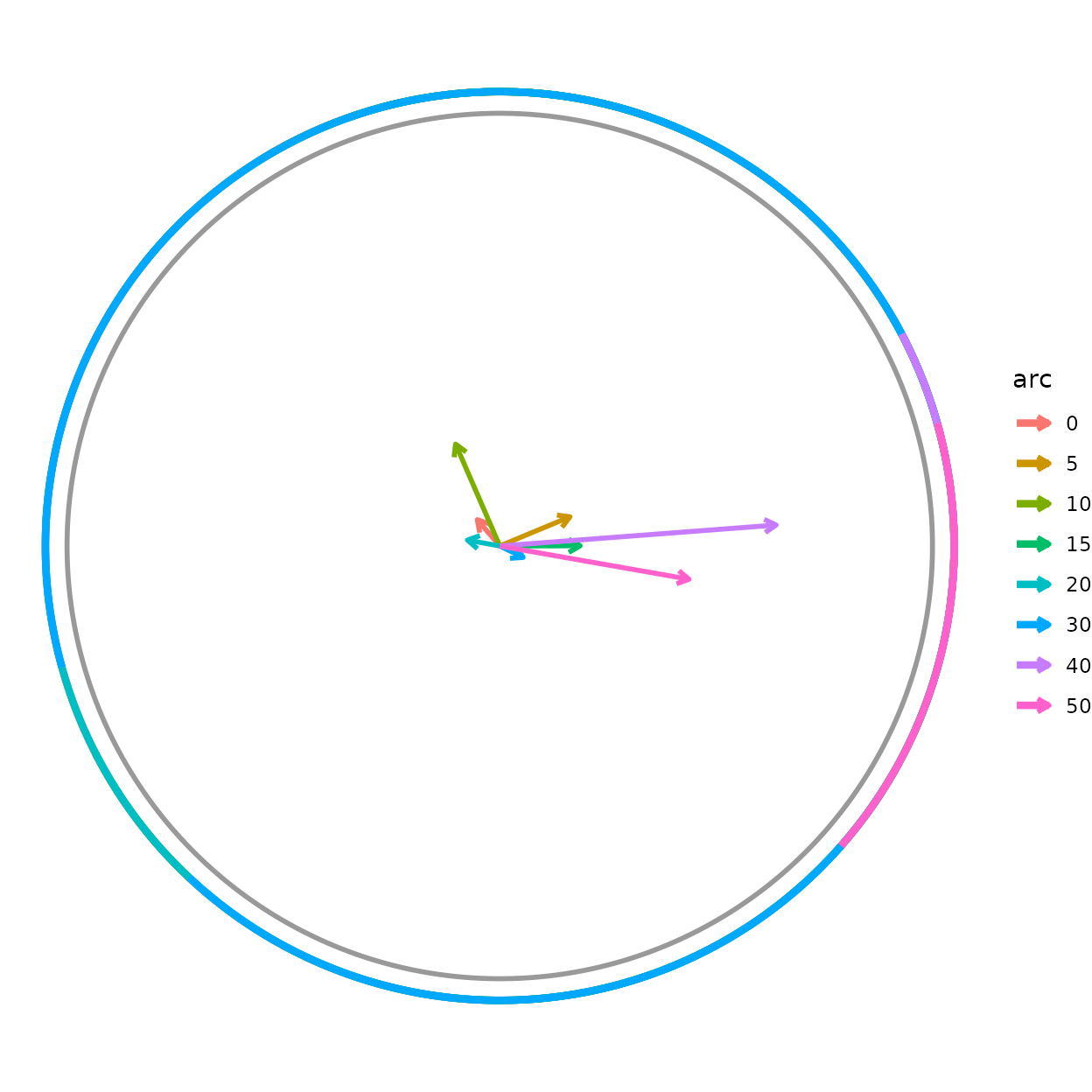

Each arc group gets its own mean vector and CI arc in a matching colour. The grouping is independent of any faceting, so you can (for example) colour by cohort while faceting radiate() by treatment. radiate()’s own built-in arrow follows the same idea via arrow_colour_col, drawing one arrow per group:

radiate(cpunctatus, group_col = "trial_id",
        show_arrow = TRUE, arrow_colour_col = "arc")

Significance geometry

The remaining two helpers draw the decision boundary of a significance test directly in resultant-length space (radius 0–1), so it can be read against the observed mean vector.

add_critical_r() draws the Rayleigh critical circle: the mean resultant length needed for significance at level alpha, namely $r_\text{crit} = \sqrt{-\log(\alpha)/n}$ . If the mean vector reaches past the circle, the headings are significantly non-uniform.

disp <- circ_dispersion(hd)
mean_vec <- data.frame(x = disp$resultant_R * cos(disp$mean_dir),
                       y = disp$resultant_R * sin(disp$mean_dir))

canvas +
  add_critical_r(hd, alpha = 0.05, test = "rayleigh") +
  geom_segment(data = mean_vec,
               aes(x = 0, y = 0, xend = x, yend = y),
               arrow = arrow(length = unit(0.15, "inches")),
               linewidth = 1)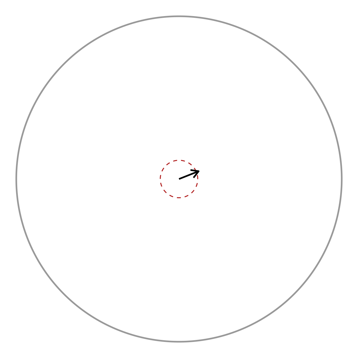

test_uniformity(hd, test = "rayleigh")
#>   statistic    p_value   n     test
#> 1 0.1298181 0.02217652 226 rayleigh

The arrow tip lies well outside the dashed critical circle, matching the tiny Rayleigh p-value above.

add_critical_v_line() is the corresponding boundary for the V-test, which tests uniformity against a specified direction mu0 (here 0, i.e. toward the target). Unlike the Rayleigh circle, the V-test boundary is a straight line perpendicular to mu0: significance requires the mean vector’s projection onto mu0 to exceed $c = z_\alpha / \sqrt{2n}$ . Set show_region = TRUE to shade the rejection side.

canvas +
  add_critical_v_line(hd, mu0 = 0, alpha = 0.05, show_region = TRUE) +
  geom_segment(data = mean_vec,
               aes(x = 0, y = 0, xend = x, yend = y),
               arrow = arrow(length = unit(0.15, "inches")),
               linewidth = 1)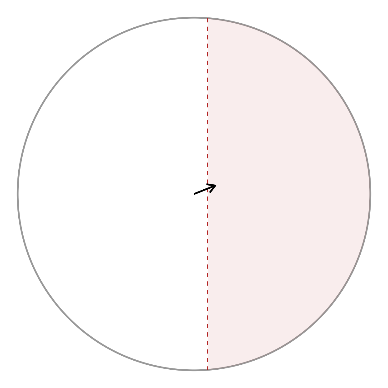

When the experiment has an a priori expected direction (the target), the V-test is more powerful than the omnibus Rayleigh test, and the line makes the one-sided nature of the decision visible.

Where next

The main vignette covers building these heading data frames and the trajectory/heading-overlay plotting layers.
The Loaders vignette covers reading tracking exports from 20+ tools into the TrajSet objects these analyses start from.
Every function above is documented individually under Reference, grouped by role (summaries, parametric fitting, correlation, hypothesis tests, and distribution overlays). ```