if (requireNamespace("pkgload", quietly = TRUE)) {
  pkgload::load_all("..", export_all = FALSE, helpers = FALSE, quiet = TRUE)
} else if (requireNamespace("radiatR", quietly = TRUE)) {
  library(radiatR)
} else {
  stop("Package 'radiatR' not installed and 'pkgload' not available.")
}
library(ggplot2)
Overview
simulate_tracks() generates synthetic trajectories on
the unit disk without any tracking files. Its main uses are:
- Verifying that a new analysis pipeline works before real data arrives.
- Reproducing plots and examples in documentation.
- Teaching: demonstrating how concentration, tortuosity, and directional bias each affect the appearance of paths.
- Informal power analysis: generate data under a plausible effect size and check whether the expected statistical pattern is visible.
Quick Start
Called with no arguments, simulate_tracks() returns a
tibble of three conditions (60 trials total, 200 frames each):
sim <- simulate_tracks(seed = 1)
dim(sim)
#> [1] 12000    24
names(sim)
#>  [1] "condition"     "trial_id"      "trial_num"     "frame"
#>  [5] "predictor"     "concentration" "tortuosity"    "ref_heading"
#>  [9] "final_heading" "rho"           "abs_theta"     "rel_theta"
#> [13] "abs_x"         "abs_y"         "rel_x"         "rel_y"
#> [17] "modality"      "n_modes"       "mode_id"       "mode_mean"
#> [21] "track_shape"   "n_reversals"   "amplitude"     "line_width"
Each row is one frame. The key columns are:
| Column | Description |
|---|---|
condition |
Condition label |
trial_id |
Unique trial identifier
(<condition>_<index>) |
frame |
Frame number within the trial |
predictor |
Per-trial continuous covariate value |
concentration |
Effective von Mises κ for the trial |
tortuosity |
Effective angular noise σ for the trial |
final_heading |
Drawn heading (unit-circle radians) |
abs_x, abs_y
|
Absolute position on the unit disc |
rel_x, rel_y
|
Position re-centred on the heading direction |
abs_theta, rel_theta
|
Corresponding angular coordinates |
Output Formats
The output argument controls what is returned.
# Default: long-form tibble
sim_tbl  <- simulate_tracks(seed = 1, output = "tibble")

# Tracks directly (ready for radiate(), derive_headings(), etc.)
sim_ts   <- simulate_tracks(seed = 1, output = "trajset")

# Both representations in a named list
sim_both <- simulate_tracks(seed = 1, output = "both")
names(sim_both)  # "tibble" "trajset"
The output = "trajset" path wraps the tibble in a
Tracks (absolute coordinates, no normalisation). Use it
whenever you want to plug straight into the plotting or analysis
functions.
Plotting the Default Simulation
ts_default <- simulate_tracks(seed = 1, output = "trajset")
radiate(ts_default,
        group_col    = "trial_id",
        colour_cycle = 10,
        facets     = "condition",
        ncol         = 3,
        show_labels  = FALSE,
        show_arrow   = TRUE)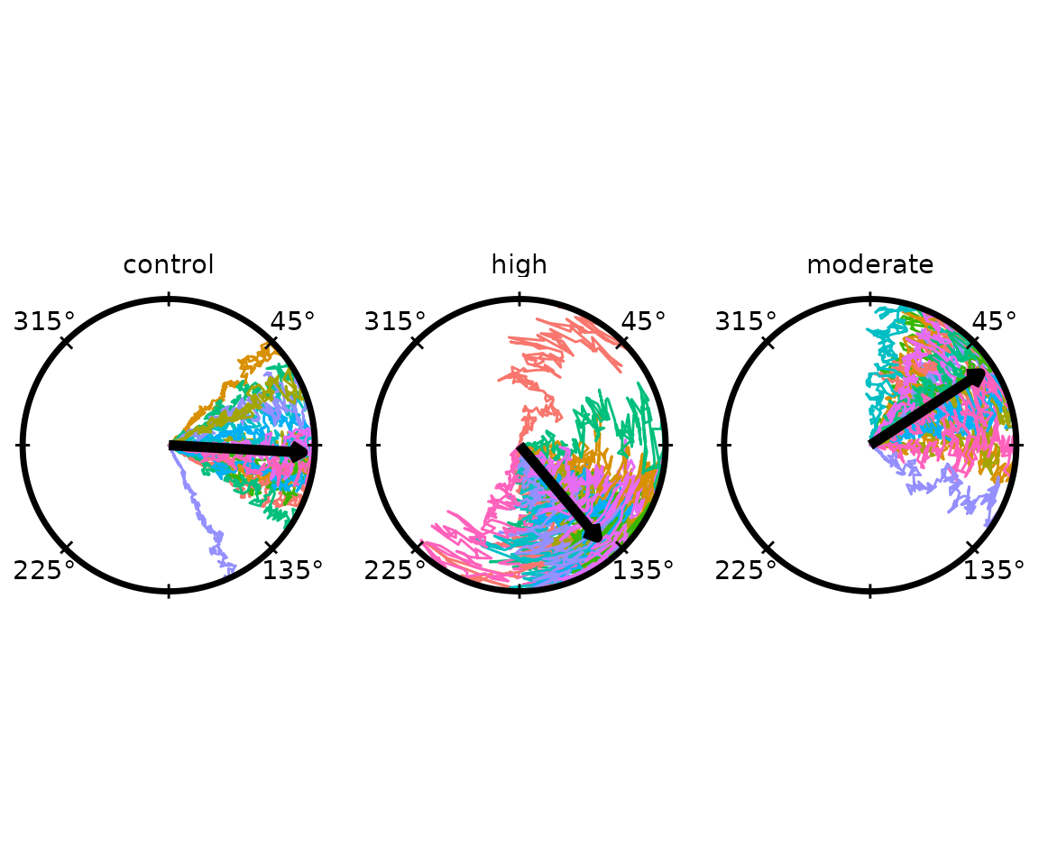
The three default conditions differ in directional bias, concentration, and tortuosity (see below).
The Conditions Table
All simulation behaviour is controlled by a data frame passed to
conditions. When conditions = NULL the
function fills in a three-condition template. Supply your own data frame
to override any subset of columns; missing columns receive sensible
defaults.
| Column | Default | Description |
|---|---|---|
condition |
"condition_N" |
Label for the condition |
n_trials |
10 |
Number of trajectories |
ref_mean |
0 |
Baseline reference direction (unit-circle radians) |
concentration_base |
5 |
Baseline von Mises κ |
concentration_slope |
0 |
Slope of κ on the per-trial predictor |
tortuosity_base |
0.06 |
Baseline angular noise σ |
tortuosity_slope |
0 |
Slope of σ on the predictor |
tortuosity_sd |
0.01 |
Trial-to-trial variability in σ |
predictor_mean |
0 |
Mean of the per-trial predictor distribution |
predictor_sd |
0.2 |
SD of the predictor distribution |
predictor_values |
(none) | Optional list-column of explicit predictor values |
Concentration (κ)
concentration_base is the von Mises κ passed to
rvonmises(). Higher values produce tightly clustered
headings; values near zero produce near-uniform heading
distributions.
conds_kappa <- data.frame(
  condition          = c("low (κ=0.1)", "medium (κ=1)", "high (κ=12)"),
  n_trials           = 20L,
  concentration_base = c(0.1, 1, 12),
  tortuosity_base    = 0.05
)
ts_kappa <- simulate_tracks(conditions = conds_kappa, seed = 42,
                             output = "trajset")
radiate(ts_kappa,
        group_col    = "trial_id",
        colour_cycle = 10,
        facets     = "condition",
        ncol         = 3,
        show_labels  = FALSE,
        show_arrow   = TRUE)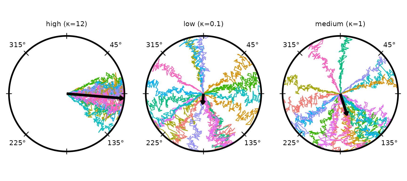
At κ = 1 the mean arrow is short (low resultant length); at κ = 12 nearly all trials point in the same direction.
Tortuosity and Path Smoothness
Two parameters control within-trial path shape:
-
tortuosity_base— the SD of the per-step angular noise. Larger values produce more sinuous paths. -
phi— autocorrelation of successive angular deviations (0 = white noise, values near 1 produce smooth, sweeping curves). Passed directly tosimulate_tracks(), not via the conditions table.
conds_tort <- data.frame(
  condition          = c("smooth (φ=0.95)", "moderate (φ=0.7)", "noisy (φ=0)"),
  n_trials           = 15L,
  concentration_base = 6,
  tortuosity_base    = c(0.12, 0.12, 0.12)
)
phi_vals <- c(0.95, 0.7, 0)

# Simulate each phi separately and bind
parts <- lapply(seq_along(phi_vals), function(i) {
  d <- conds_tort[i, , drop = FALSE]
  simulate_tracks(conditions = d, n_points = 200,
                  phi = phi_vals[i], seed = 7 + i)
})
ts_tort <- tracks(
  do.call(rbind, parts),
  id = "trial_id", time = "frame",
  x = "abs_x", y = "abs_y", angle = "abs_theta",
  angle_unit = "radians", normalize_xy = FALSE
)
radiate(ts_tort,
        group_col    = "trial_id",
        colour_cycle = 10,
        facets     = "condition",
        ncol         = 3,
        show_labels  = FALSE,
        show_arrow   = FALSE)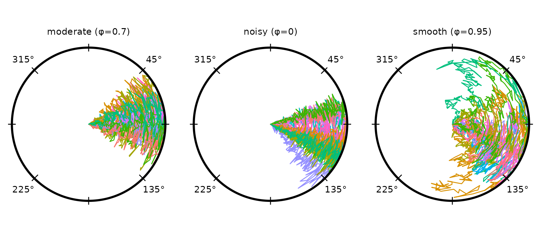
Directional Bias (ref_mean)
ref_mean shifts the reference direction away from East
(0 rad). Use it to simulate experiments where the reference is not along
the positive x-axis.
conds_bias <- data.frame(
  condition          = c("East (0°)", "North (90°)", "Northwest (135°)"),
  n_trials           = 20L,
  concentration_base = 5,
  tortuosity_base    = 0.06,
  ref_mean          = c(0, pi / 2, 3 * pi / 4)
)
ts_bias <- simulate_tracks(conditions = conds_bias, seed = 99,
                           output = "trajset")
radiate(ts_bias,
        group_col    = "trial_id",
        colour_cycle = 10,
        facets     = "condition",
        ncol         = 3,
        show_labels  = FALSE,
        show_arrow   = TRUE)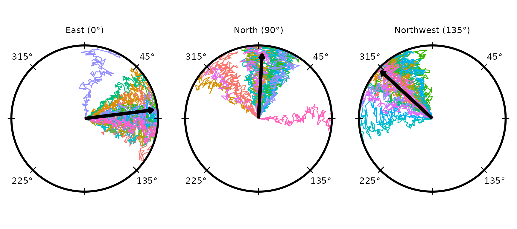
Multi-Condition Gradient
A common design is a monotone gradient in cue strength. The example below simulates four levels with increasing concentration and decreasing tortuosity — mimicking an orientation experiment where stronger cues produce tighter, smoother paths.
conds_grad <- data.frame(
  condition          = paste0(c(15, 30, 60, 120), "° arc"),
  n_trials           = 25L,
  concentration_base = c(1.5, 3, 6, 10),
  tortuosity_base    = c(0.14, 0.10, 0.06, 0.03),
  tortuosity_sd      = 0.015
)
ts_grad <- simulate_tracks(conditions = conds_grad, n_points = 200,
                            seed = 55, output = "trajset")
radiate(ts_grad,
        group_col    = "trial_id",
        colour_col   = "condition",
        facets     = "condition",
        ncol         = 4,
        show_labels  = FALSE,
        show_arrow   = TRUE)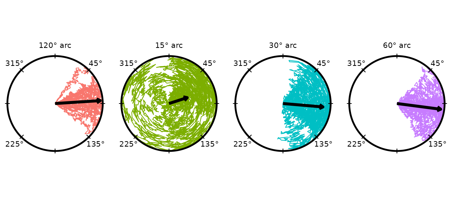
Continuous Predictor
When concentration_slope or
tortuosity_slope is non-zero, the final kappa and
tortuosity of each trial depend on its sampled predictor value. This
lets you model experiments where individual differences (e.g. body size,
prior exposure) modulate the response.
conds_pred <- data.frame(
  condition            = "gradient",
  n_trials             = 40L,
  concentration_base   = 3,
  concentration_slope  = 4,    # kappa rises with predictor
  tortuosity_base      = 0.10,
  tortuosity_slope     = -0.04, # smoother at high predictor
  predictor_mean       = 0,
  predictor_sd         = 1
)
sim_pred <- simulate_tracks(conditions = conds_pred, seed = 7, output = "both")

# Each trial gets its own predictor sample
range(sim_pred$tibble$predictor)
#> [1] -1.387996  2.716752
range(sim_pred$tibble$concentration)
#> [1]  0.10000 13.86701
Plotting concentration against the predictor confirms the linear relationship:
trial_summary <- unique(sim_pred$tibble[, c("trial_id", "predictor",
                                             "concentration")])
ggplot(trial_summary, aes(predictor, concentration)) +
  geom_point(alpha = 0.5) +
  geom_smooth(method = "lm", se = FALSE, colour = "steelblue") +
  labs(x = "Predictor", y = "Effective κ") +
  theme_minimal()
#> `geom_smooth()` using formula = 'y ~ x'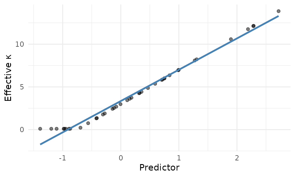
Connecting to Circular Analysis
Simulated Tracks objects feed directly into
derive_headings() and circ_summarise(), making
it straightforward to run the same analysis pipeline on synthetic
data.
conds_analysis <- data.frame(
  condition          = c("diffuse", "concentrated"),
  n_trials           = 30L,
  concentration_base = c(1.5, 8),
  tortuosity_base    = c(0.12, 0.04)
)
sim_analysis <- simulate_tracks(conditions = conds_analysis, seed = 21,
                                 output = "both")

hd <- derive_headings(sim_analysis$trajset, rule = "crossing",
                       circ0 = 0.2, circ1 = 0.4,
                       coords = "absolute",
                       angle_convention = "unit_circle",
                       return_coords = TRUE)
names(hd)[names(hd) == "id"] <- "trial_id"

# derive_headings returns only id/heading/coords; join condition back
cond_map <- unique(sim_analysis$tibble[, c("trial_id", "condition")])
hd <- merge(hd, cond_map, by = "trial_id")

compute_circ_mean(hd, group_col = "condition")[,
  c("condition", "mean_dir", "resultant_R")]
#>      condition   mean_dir resultant_R
#> 1 concentrated 0.05301978   0.9039690
#> 2      diffuse 0.29012285   0.7131608
Visualise the headings alongside the trajectories:
p <- radiate(sim_analysis$trajset,
             group_col    = "trial_id",
             colour_col   = "condition",
             facets     = "condition",
             ncol         = 2,
             show_labels  = FALSE,
             show_arrow   = FALSE) +
  add_heading_points(hd, colour_col = "condition", size = 2, alpha = 0.7) +
  add_heading_arrow(hd, colour_col = "condition", colour = "black")
p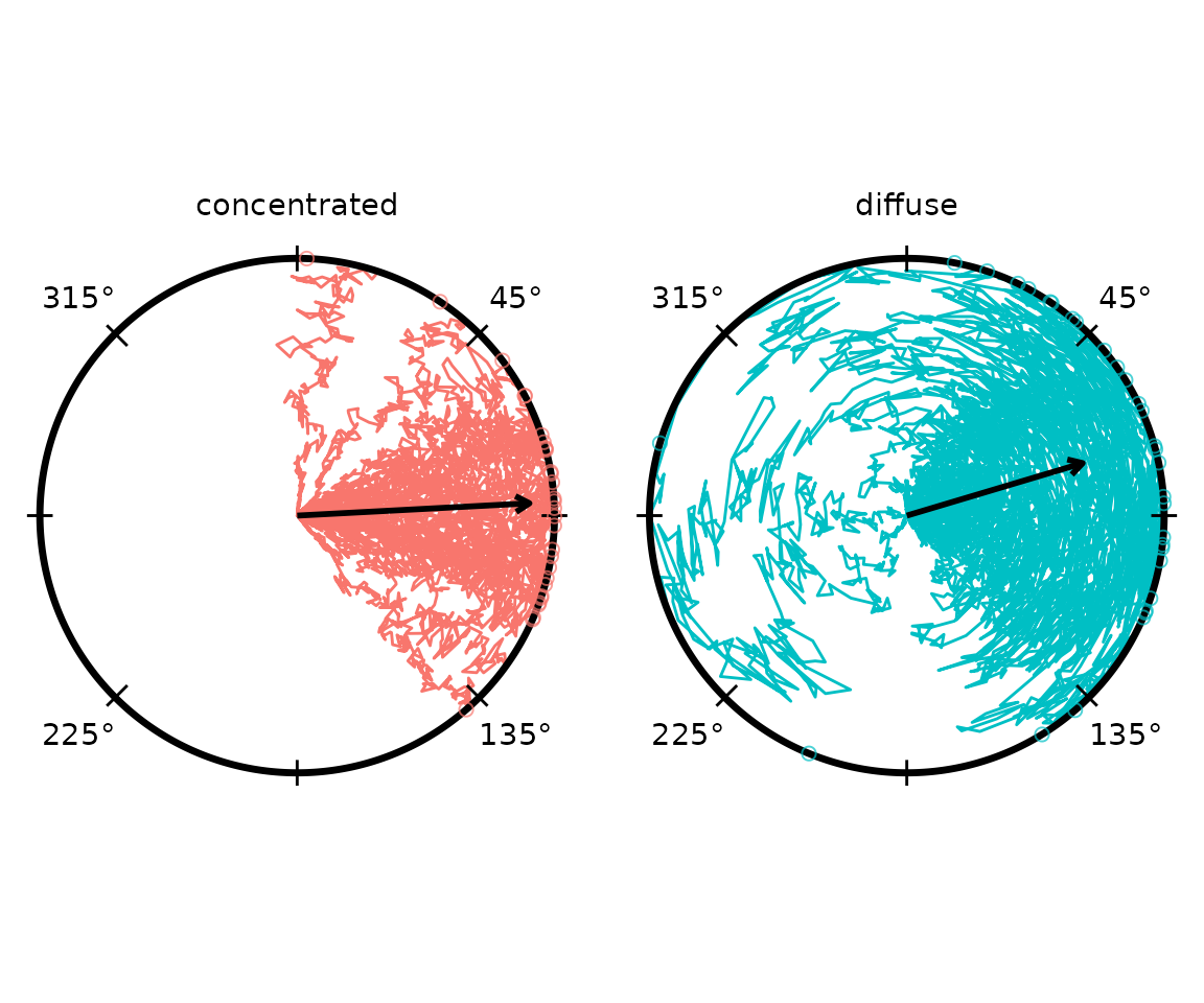
Known Modality and Shape
simulate_tracks() can also attach a known directional
ground truth, which is handy for sanity-checking the circular
statistics: you know what the analysis should recover. The
modality of a condition sets how its per-trial principal
headings are distributed — uniform (no preferred
direction), unimodal (one von Mises mode),
axial (two antipodal modes), or multimodal
(n_modes evenly spaced modes). Here one condition per
modality, fed through a directional heading rule (net) and
circ_model_select(), recovers the generating model:
conds <- tibble::tibble(
  condition          = c("uniform", "unimodal", "axial"),
  n_trials           = 60L,
  ref_mean           = 0.4,
  concentration_base = 6,
  modality           = c("uniform", "unimodal", "axial")
)
sim <- simulate_tracks(conditions = conds, n_points = 80,
                       output = "both", seed = 7)

# net heading per trial, with the condition label joined back on
hd <- derive_headings(sim$trajset, rule = "net")
names(hd)[names(hd) == "id"] <- "trial_id"
hd <- merge(hd, unique(sim$tibble[, c("trial_id", "condition")]),
            by = "trial_id")

# best-supported model per condition (AICc; lowest dAICc = best)
ms <- circ_model_select(hd, group_col = "condition")
do.call(rbind, lapply(split(ms, ms$condition), function(d) {
  d[which.min(d$AICc), c("condition", "model", "weight")]
}))
#>          condition    model    weight
#> axial        axial    axial 0.8243673
#> uniform    uniform unimodal 0.3306096
#> unimodal  unimodal unimodal 0.7256195
The unimodal and axial conditions are
picked out cleanly (Akaike weight near 1); the uniform
condition leaves uniform and unimodal in a near-tie,
as it should when there is no preferred direction to fit.
The track_shape of a condition sets the
within-track geometry instead. A
track_shape = "oscillatory" condition produces
back-and-forth tracks along a principal axis — the bidirectional pattern
the per-track axial methods are built for. The oscillatory tracks form a
genuinely axial position cloud, so the position-based estimator
pca_axis recovers the axis at the default sampling density,
while a directional rule (net) sees the to-and-fro
directions cancel:
osc <- tibble::tibble(condition = "osc", n_trials = 40L, ref_mean = 0.6,
                      concentration_base = 50, track_shape = "oscillatory",
                      n_reversals = 4L)
ts_osc <- simulate_tracks(conditions = osc, output = "trajset", seed = 11)

# pca_axis recovers the ~0.6 rad axis (read it as an axial mean) at defaults
pa <- derive_headings(ts_osc, rule = "pca_axis")
circ_summarise(pa, "heading", axial = TRUE, units = "radians",
               stats = "mean_dir")
#> # A tibble: 1 × 1
#>   mean_dir
#>      <dbl>
#> 1    0.611

# net cannot: the directions cancel to a tiny resultant length
net <- derive_headings(ts_osc, rule = "net")
circ_summarise(net, "heading", units = "radians", stats = "resultant_R")
#> # A tibble: 1 × 1
#>   resultant_R
#>         <dbl>
#> 1       0.152
The oscillatory line-width (line_width) is a fixed
fraction of the amplitude, independent of tortuosity_base,
so the axis is recoverable at the default settings used here without any
signal-to-noise tuning. Note the position-based methods
(pca_axis, ransac_straight) are the robust
choice: the step-based velocity_axis recovers the same axis
only at coarse sampling, because its per-step axial signal shrinks with
n_points while the perpendicular jitter step does not, so
dense sampling lets the jitter flip the estimate toward the
perpendicular.
Reproducibility and Saving
Pass seed for exact reproducibility. Pass
write_path to write the tibble to a CSV alongside (or
instead of) returning it — useful when you want to hand the data to a
colleague or another tool.
simulate_tracks(
  conditions = conds_grad,
  n_points   = 200,
  seed       = 55,
  write_path = "sim_gradient.csv"
)