Wrap a pre-computed circular density around the unit circle

Takes a data frame of `(theta, density)` pairs – from any source: MLE, kernel estimation, Bayesian posterior predictive, or hand-crafted – and renders it as a radial path (and optionally a filled polygon) around the unit circle boundary. At each angle theta the plotted radius is `1 + scale * density(theta) / max(density)`.

Usage

add_circular_density(
  density_df,
  theta_col = "theta",
  density_col = "density",
  colour_col = NULL,
  scale = 0.4,
  colour = "black",
  fill = NA,
  alpha = 0.2,
  linewidth = 0.8,
  ci_fill = "grey70",
  ci_alpha = 0.3
)

Arguments

density_df: Data frame with columns named by `theta_col` and `density_col` (and, optionally, `colour_col`). Each row represents one evaluated angle.
theta_col: Name of the angle column (radians, -pi to pi). Default `"theta"`.
density_col: Name of the density/count column. Default `"density"`.
colour_col: Optional grouping column. When set, separate paths are drawn per group, enabling ggplot2 faceting.
scale: Maximum radial extension above the unit circle. Default `0.4` (peak at r = 1.4). Density is normalised within each group before scaling.
colour: Fixed line colour used when `colour_col` is `NULL`. Default `"black"`.
fill: Colour for the region between the unit circle and the density curve. `NA` (default) draws no fill.
alpha: Alpha transparency for the filled polygon. Default `0.2`.
linewidth: Width of the density path. Default `0.8`.
ci_fill: Fill colour for the bootstrap confidence band. Only used when `density_df` contains `density_lower` and `density_upper` columns (produced by [compute_circular_density()] with `boot_reps > 0`, or supplied manually). Default `"grey70"`.
ci_alpha: Alpha transparency for the confidence band polygon. Default `0.3`.

Value

A list of one, two, or three ggplot2 layers: optional CI band polygon, optional fill polygon between density and unit circle, and density path line.

Details

Because this function only handles rendering, it is agnostic to how the density was produced. To compute from raw headings use [compute_circular_density()] first, or call the convenience wrapper [add_heading_density()] which combines both steps.

Examples

library(ggplot2)
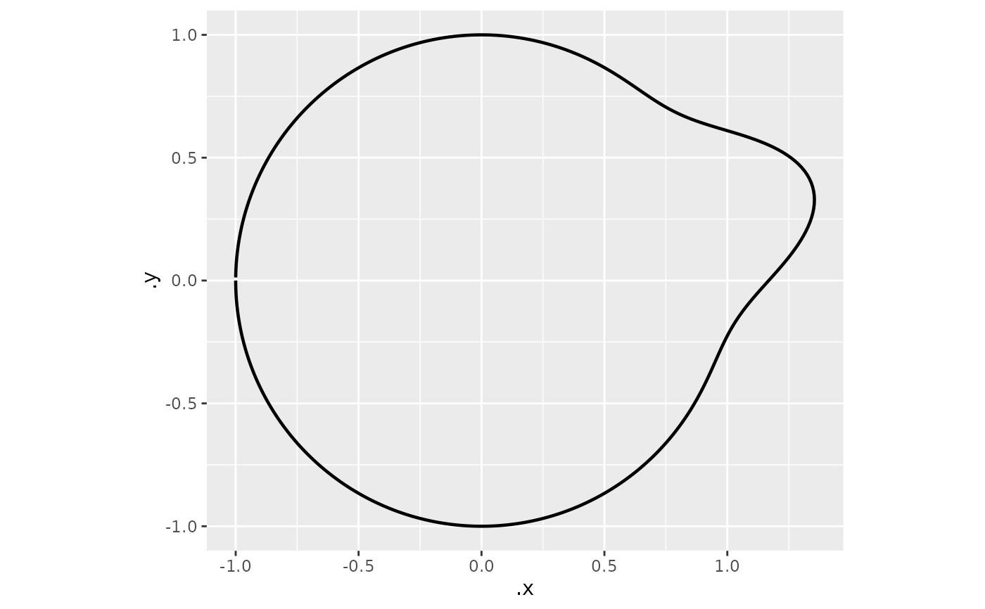
# From compute_circular_density:
hd <- data.frame(heading = c(0.2, 0.3, 0.4, 0.5, -0.1, 0.1, 0.6, 0.2))
dens_df <- compute_circular_density(hd)
ggplot() + coord_fixed() + add_circular_density(dens_df)


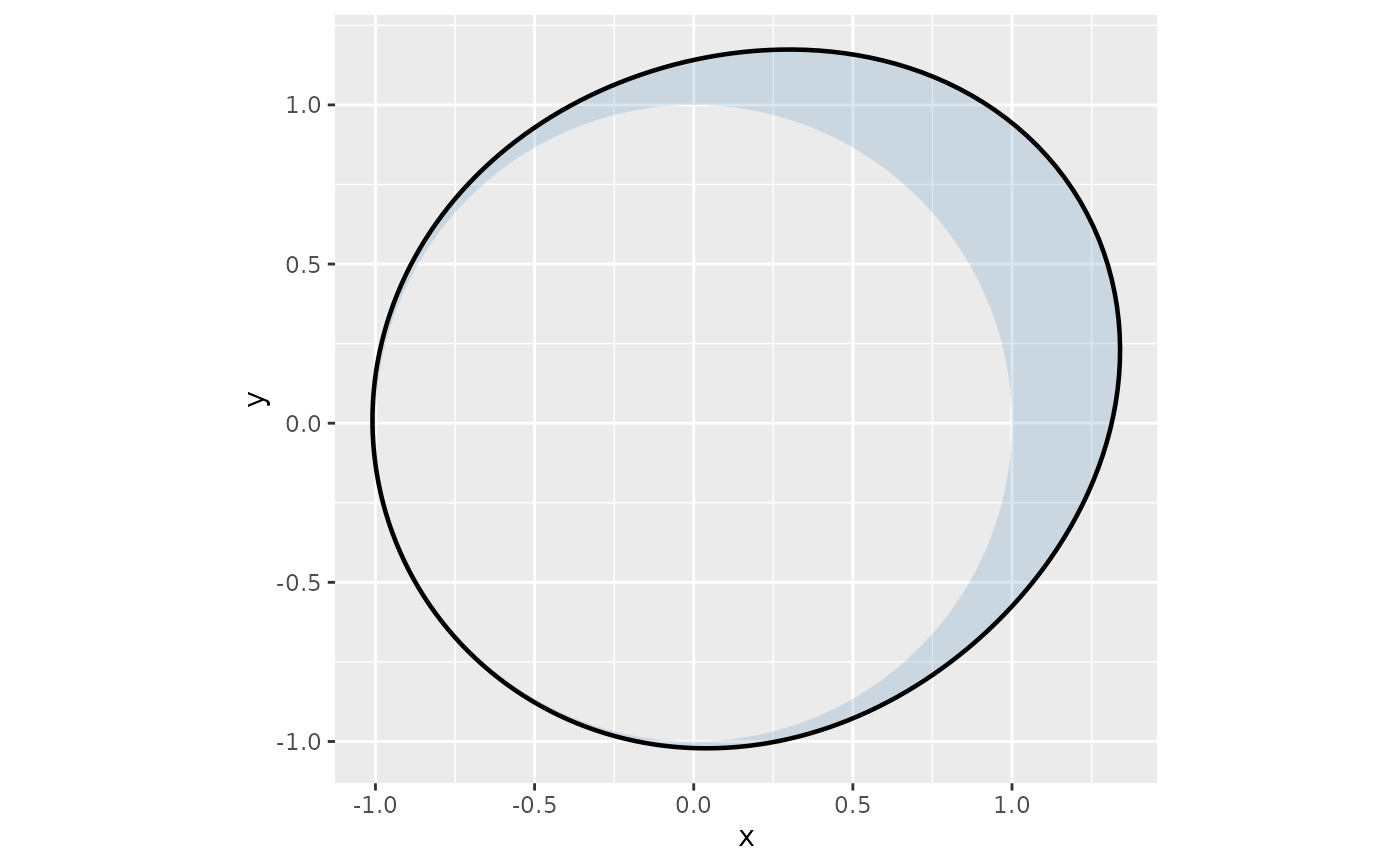
# From an external model (e.g. brms posterior predictive):
theta_grid <- seq(-pi, pi, length.out = 200)
external_dens <- data.frame(
  theta   = theta_grid,
  density = exp(-2 * (1 - cos(theta_grid - 0.5)))  # von Mises-like
)
ggplot() + coord_fixed() + add_circular_density(external_dens, fill = "steelblue")