Seeing through water: from sunlight to detection • luxR

This vignette runs a single question end to end: can a fish, at depth, detect a reddish object against the open-water background — and how far away? It chains the three stages luxR is built around:

Sunlight to depth — cross the air–water surface and attenuate the solar spectrum through a Jerlov water type.
Light to capture — what the fish’s photoreceptors actually catch, allowing for self-screening.
Capture to detection — the inherent object/background contrast and the distance at which it falls below threshold.

library(luxR)

1. Sunlight to depth

Start with the clear-noon solar spectrum just above the surface. A flat air–water interface reflects a few percent of it away (Fresnel); surface_transmittance() gives the fraction that actually enters the water.

sp    <- solar_irradiance("clear_noon")   # W/m2/nm, above surface
lam   <- sp$wavelength

tau   <- surface_transmittance(angle = 30)            # sun 30 deg from vertical
E_sub <- sp$irradiance * tau                          # just below the surface
round(tau, 3)

## [1] 0.979

Now propagate that subsurface spectrum down through Jerlov type II water with Beer–Lambert attenuation. The water is a strong spectral filter: red light is gone within a few metres, leaving a blue-green field at depth.

depth  <- 10                                          # metres
at_10m <- light_at_depth("clear_noon", "II", depth,
                         wavelength_policy = "trim",
                         surface_source = "direct", surface_angle = 30)
lam_depth <- at_10m$lambda
supported <- lam >= min(lam_depth) & lam <= max(lam_depth)
E_10m  <- at_10m$irradiance
E_sub <- E_sub[supported]
lam <- lam_depth

plot(lam, E_sub, type = "l", col = "goldenrod", lwd = 2,
     xlab = "Wavelength (nm)", ylab = "Irradiance (W/m2/nm)",
     main = "Surface vs 10 m (Jerlov II)")
lines(lam, E_10m, col = "steelblue4", lwd = 2)
legend("topright", c("Just below surface", "10 m"),
       col = c("goldenrod", "steelblue4"), lwd = 2, bty = "n")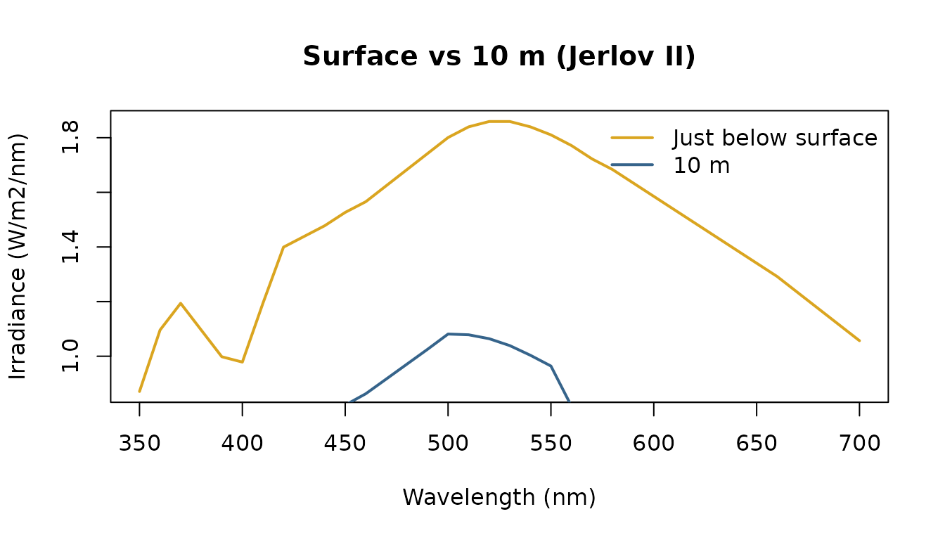

2. Light to capture

Here, quantum catch means the in-water photon irradiance weighted by the receptor’s spectral sensitivity. It remains an area-normalised quantity, not an absolute per-receptor photon rate. The sensitivity itself is not the bare pigment template — a real outer segment is partly self-screening, which broadens the effective curve. receptor_absorptance() applies that for a chosen axial optical density.

viewer <- "Danio rerio"                               # a tetrachromat
recs   <- unique(subset(species_sensitivities,
                        species == viewer)$receptor)

lam_s  <- seq(300, 750, by = 1)
catch  <- sapply(recs, function(r) {
  row <- subset(species_sensitivities,
                species == viewer & receptor == r)
  tmpl <- govardovskii_template(lam_s, row$lambda_max[1], row$chromophore[1])
  S    <- receptor_absorptance(tmpl, optical_density = 0.4)   # self-screening
  quantum_catch(E_10m, lam, S, input_unit = "W/m2/nm")
})
round(catch)

##      UV-cone       S-cone       M-cone       L-cone 
## 2.165623e+19 6.750210e+19 1.459543e+20 1.677082e+20

The catches span almost an order of magnitude across the four cones — a direct readout of how much each receptor’s sensitivity overlaps the residual blue-green field at depth, rather than the broad, even excitation it would receive at the surface.

3. Capture to detection

Now the target. Give it a reddish reflectance and view it against a flat grey background under the 10 m light field. inherent_contrast() returns both an achromatic (brightness) Weber contrast and a chromatic distance (ΔS, in JNDs) for the viewer’s receptors.

grey <- rep(0.30, length(lam))
red  <- 0.20 + 0.25 * exp(-((lam - 625) / 35)^2)

ic <- inherent_contrast(red, grey, E_10m, lam, species = viewer)
ic

## $achromatic
## [1] -0.2622355
## 
## $chromatic
## [1] 1.743446

The default scenario assumes both scalar contrasts decay with distance as veiling light replaces the object (C(r) = C0 * exp(-c r)). This is a teaching heuristic, not an empirically validated prediction of an animal’s actual detection range. detectability() bundles the inherent contrast, the threshold-distance estimate per channel, and the contrast-vs-distance curve. We pass a real beam attenuation c = a + b rather than the Kd * kd_to_c proxy.

c_beam <- beam_attenuation(absorption = 0.20, scattering = 0.12)   # 1/m
Kd_ref <- jerlov_Kd("II", lambda = 490)

d <- detectability(red, grey, E_10m, lam, Kd = Kd_ref,
                   beam_c = c_beam, species = viewer)
d

## <lux_detection> horizontal viewing, Danio rerio 
##   model: scalar contrast/JND heuristic scenario estimate 
##   validation: not empirically validated as an actual detection range
##   achromatic: C0 = -0.262 (Weber)   -> estimate 8.04 m  (thr 0.020; crossed)
##   chromatic : dS = 1.743 JND        -> estimate 1.74 m  (thr 1.00 JND; crossed)

plot(d)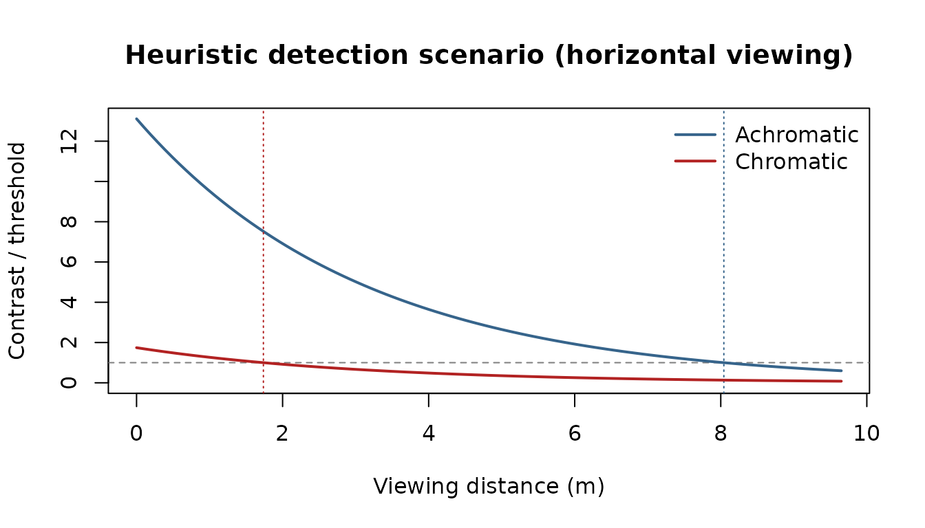

Under this heuristic the two channels behave very differently. The brightness (achromatic) difference stays above threshold for several metres, while the colour signal — only just above 1 JND at zero distance — washes out almost immediately as veiling light floods in. Detecting an object by its colour underwater is demanding: it needs both photons and inherent contrast to spare. Looking up (against the brighter surface) extends the range, because the contrast-attenuation coefficient becomes c - Kd:

detection_range(red, grey, E_10m, lam, Kd = Kd_ref, beam_c = c_beam,
                species = viewer, channel = "achromatic",
                direction = "up")$achromatic

## [1] 9.638616

For chromatic work, prefer the wavelength-resolved path model. It requires an explicit beam-attenuation spectrum and veiling radiance rather than treating a zero-distance JND as a scalar that decays exponentially. In this illustrative geometry, the grey background is also the asymptotic veiling field:

Kd_lambda <- jerlov_Kd("II", lambda = lam)
c_lambda  <- 1.5 * Kd_lambda
veil      <- grey * irradiance2radiance(E_10m, geometry = "lambertian")

d_spectral <- detectability(
  red, grey, E_10m, lam,
  Kd = Kd_lambda,
  beam_c = c_lambda,
  species = viewer,
  model = "spectral_path",
  veiling = veil,
  max_distance = 50,
  search_points = 201
)
d_spectral

## <lux_detection> horizontal viewing, Danio rerio 
##   model: spectral-path scenario estimate 
##   validation: not empirically validated as an actual detection range
##   achromatic: C0 = -0.262 (Weber)   -> estimate 28.08 m  (thr 0.020; crossed)
##   chromatic : dS = 1.743 JND        -> estimate 13.14 m  (thr 1.00 JND; crossed)

This remains a scenario estimate: the spectral calculation improves the path physics and receptor calculation, but it does not add target size, acuity, photon limits, behaviour, or empirical validation for the organism.

Summary

From a single sunlight spectrum we crossed the surface, propagated to depth, computed photoreceptor quantum catches (with self-screening), and turned the object/background spectra into a heuristic threshold-distance scenario — the full light → capture → detection chain, each step a documented luxR function.